10  OPTIONAL: Movement Data

Week 10: Cleaning and plotting animal tracking data

This is an optional tutorial for anyone working with animal tracking (telemetry) data.

Note

This tutorial is optional and not assessed, and it will not be in the exam. Work through it in your own time if tracking data are relevant to your project.

Tracking data combine location and time, so this tutorial builds on the optional time series and spatial data tutorials.

Tracking technologies

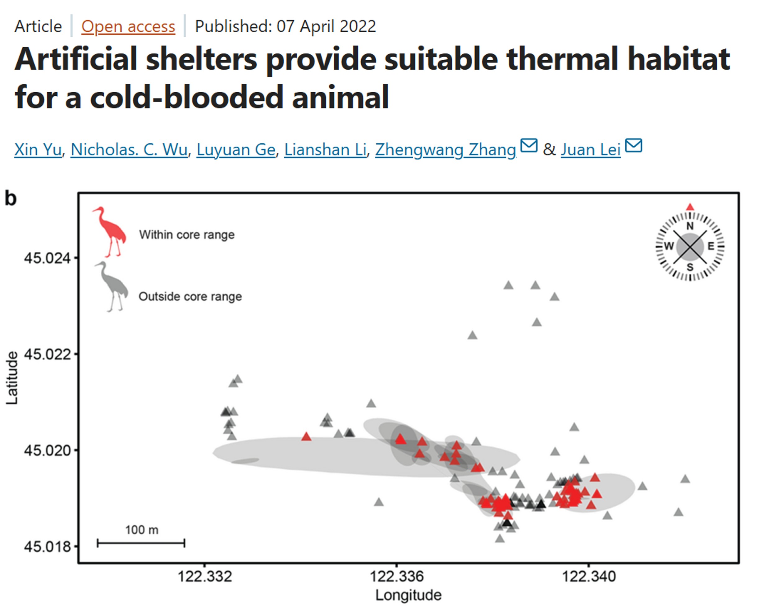
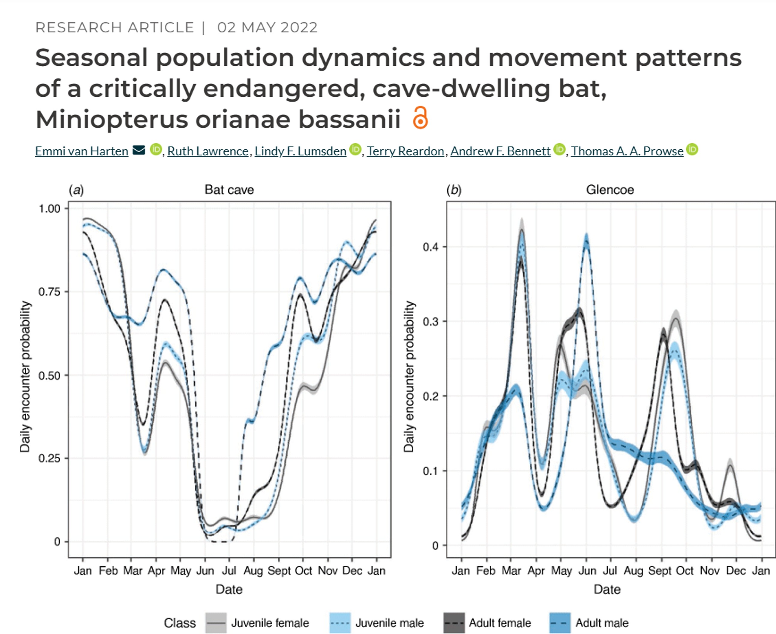
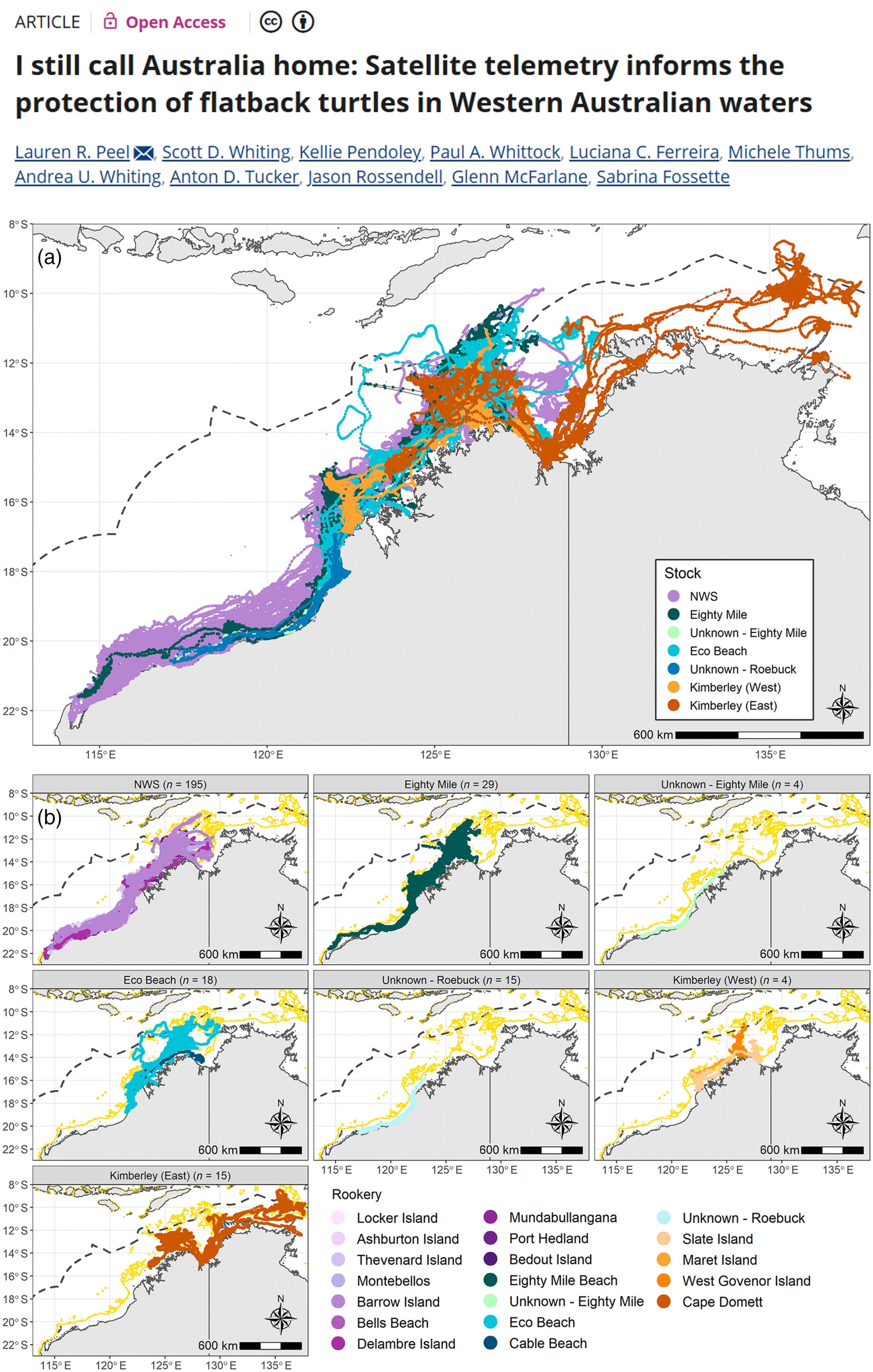
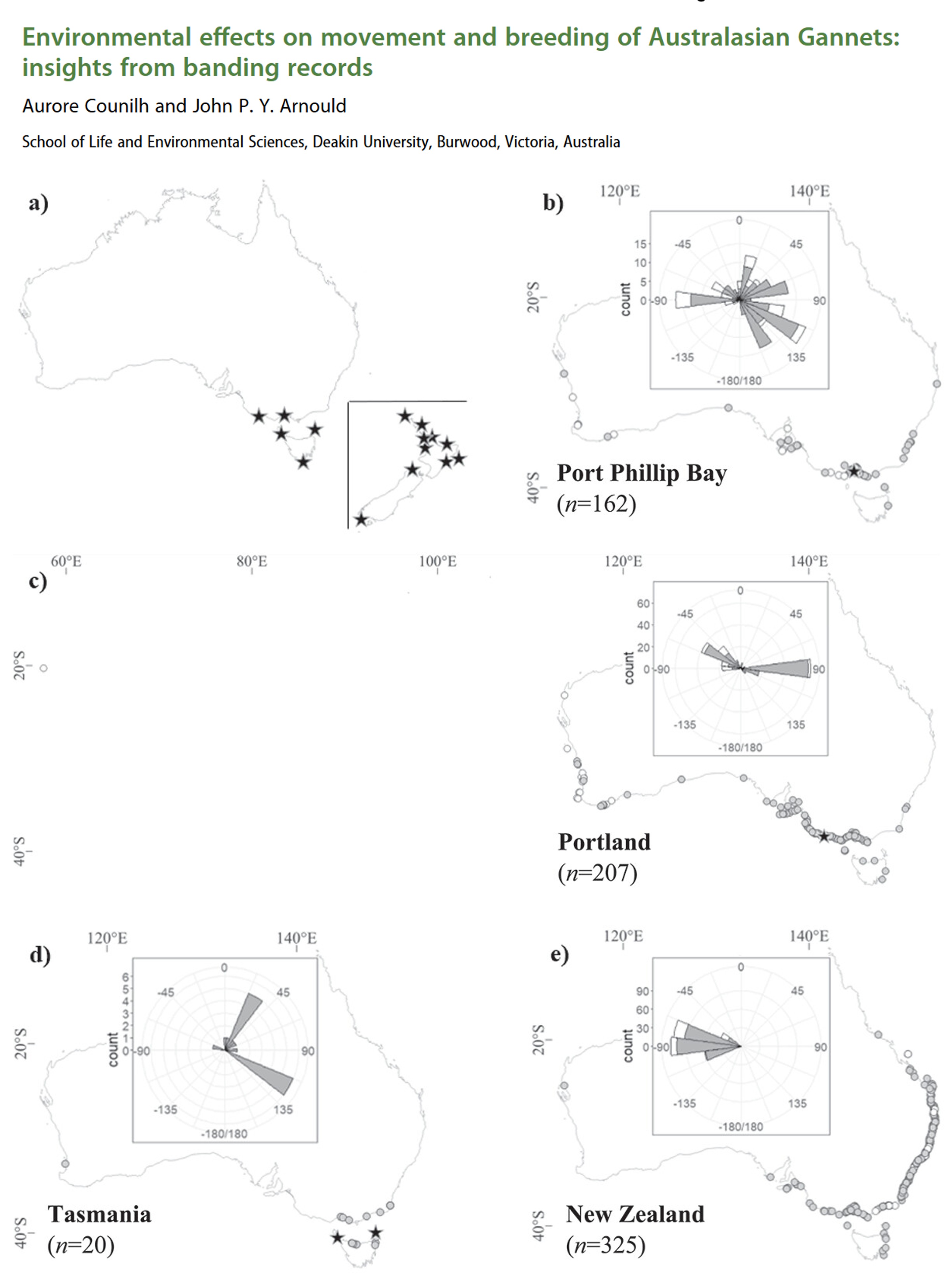
How do we track animals in the wild? There are many methods, and how you process, analyse and interpret movement data depends heavily on the method used.

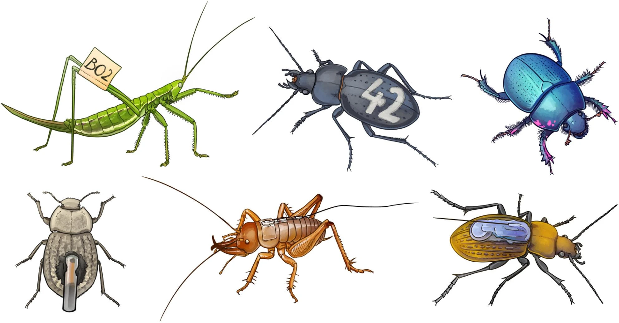
Methods for marking and tagging insects. Image from (Ržičková and Elek, 2026).

Process GPS data

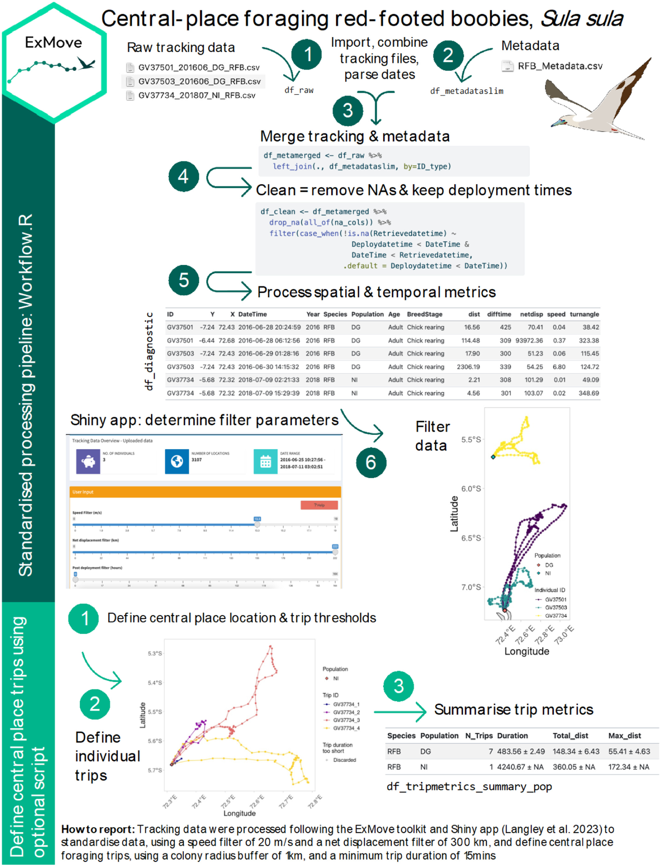
Basic tracking data contain the ID of each animal, its location (longitude and latitude) and the date and time of each location (a fix). Here we use GPS data from three red-footed boobies (Sula sula) nesting on Diego Garcia in the Indian Ocean. We loosely follow the ExMove workflow for cleaning and processing tracking data (Langley et al., 2024).

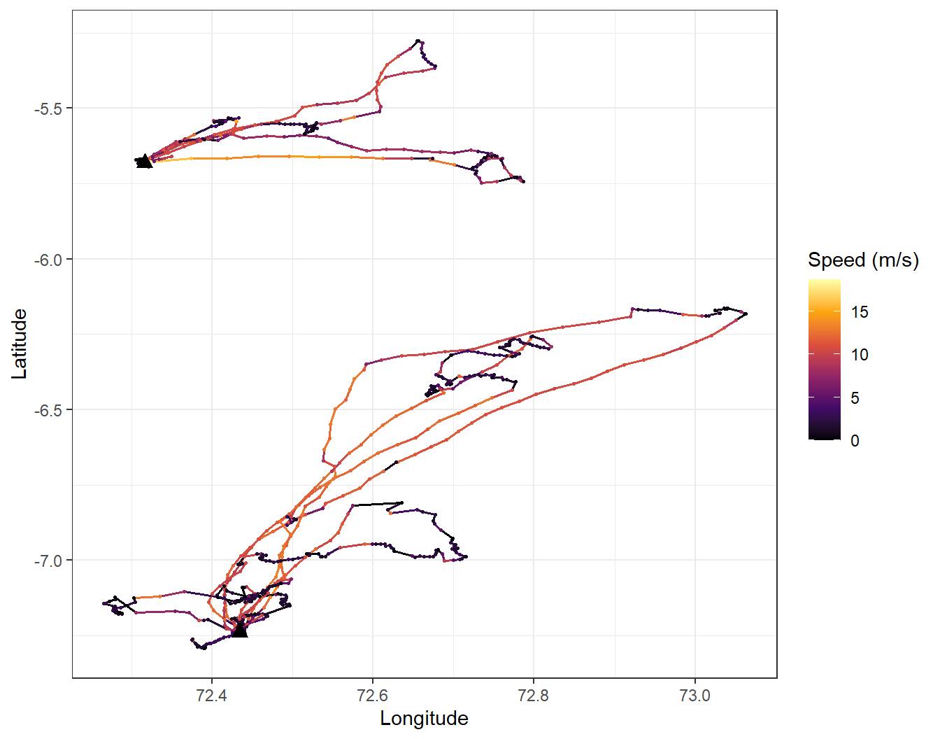
The ExMove workflow applied to GPS-tracked red-footed boobies.

Download the three GPS files and the metadata file, and save them in a folder called gps_study inside your data folder.

GV37501_201606_DG_RFB.csv GV37503_201606_DG_RFB.csv GV37734_201807_NI_RFB.csv RFB_metadata.csv

Code
# Week 10 workshop (optional) - Movement data
# Written by Nicholas Wu, 1234578, 29/04/2027

# install.packages("geosphere")  # run once in the console if needed

library(tidyverse)  # data wrangling, plotting, dates (lubridate) and text (stringr)
library(geosphere)  # distances between longitude/latitude points
library(patchwork)  # combine plots

# setwd("C:/Users/YOUR-NAME/Documents/ECS200")

Load all the GPS files

Each bird has its own file. list.files() finds them, and purrr::map() imports each one with readr::read_csv(), then purrr::list_rbind() stacks them into one data frame. id = "file_name" adds a column with the name of the file each row came from. We read Date and Time as text because the files use different date formats.

Code
# Find every file in the gps_study folder that starts with "GV" and ends in .csv
gps_files <- list.files(path = "data/gps_study", pattern = "^GV.*\\.csv$", full.names = TRUE)
gps_files
[1] "data/gps_study/GV37501_201606_DG_RFB.csv"
[2] "data/gps_study/GV37503_201606_DG_RFB.csv"
[3] "data/gps_study/GV37734_201807_NI_RFB.csv"
Code
# Import every file and stack them
gps_raw <- purrr::map(gps_files, readr::read_csv,
                      id = "file_name",
                      col_types = readr::cols(Date = "c", Time = "c")) %>%
  purrr::list_rbind()

dplyr::glimpse(gps_raw)
Rows: 6,650
Columns: 11
$ file_name <chr> "data/gps_study/GV37501_201606_DG_RFB.csv", "data/gps_study/…
$ Date      <chr> "24/06/2016", "24/06/2016", "24/06/2016", "24/06/2016", "24/…
$ Time      <chr> "05:06:00", "05:21:39", "05:29:50", "05:54:28", "06:22:02", …
$ Latitude  <dbl> -7.261829, -7.261829, -7.261744, -7.261623, -7.261651, -7.26…
$ Longitude <dbl> 72.37609, 72.37609, 72.37622, 72.37614, 72.37633, 72.37629, …
$ Altitude  <dbl> 56.18, 56.18, 64.91, -15.77, 30.91, 26.80, 21.77, 30.78, 27.…
$ Speed     <dbl> 3636, 3636, 5112, 936, 1080, 0, 0, 2844, 1476, 0, 1476, 36, …
$ Course    <dbl> 93, 93, 32, 291, 124, 280, 183, 268, 44, 260, 70, 340, 106, …
$ Type      <dbl> -2, 0, 0, 0, 0, 0, 0, 0, 0, 0, 0, 0, 0, 0, 0, 0, 0, 0, 0, 0,…
$ Distance  <dbl> 0.00, 0.00, 17.17, 16.34, 22.06, 6.26, 10.73, 1.84, 8.38, 60…
$ Essential <dbl> NA, NA, NA, NA, NA, NA, NA, NA, NA, NA, NA, NA, NA, NA, NA, …
Now tidy the columns. The bird ID is the first 7 characters of the file name (e.g. “GV37501” from “GV37501_201606_DG_RFB.csv”), which stringr::str_sub() extracts. This only works because every ID has the same length and position.

Code
gps_data <- gps_raw %>%
  dplyr::mutate(
    file_name = basename(file_name),                          # drop the folder from the name
    ID        = stringr::str_sub(file_name, start = 1, end = 7),
    Date      = lubridate::parse_date_time(Date, orders = c("dmy", "ymd")), # files use different formats
    date_time = lubridate::ymd_hms(paste(as.Date(Date), Time), tz = "GMT"),  # GPS time is in GMT
    lon       = Longitude,
    lat       = Latitude) %>%
  dplyr::select(ID, date_time, lon, lat) %>%                  # keep only the columns we need
  dplyr::arrange(ID, date_time)                               # order by bird, then time

dplyr::glimpse(gps_data)
Rows: 6,650
Columns: 4
$ ID        <chr> "GV37501", "GV37501", "GV37501", "GV37501", "GV37501", "GV37…
$ date_time <dttm> 2016-06-24 05:06:00, 2016-06-24 05:21:39, 2016-06-24 05:29:…
$ lon       <dbl> 72.37609, 72.37609, 72.37622, 72.37614, 72.37633, 72.37629, …
$ lat       <dbl> -7.261829, -7.261829, -7.261744, -7.261623, -7.261651, -7.26…

Merge with metadata

The metadata file holds one row per tag deployment: the bird ID, when the tag was attached and removed, and the nest location. These times were recorded in local time (Indian/Chagos), so we convert them to GMT to match the GPS data.

Code
meta_data <- readr::read_csv("data/gps_study/RFB_metadata.csv") %>%
  dplyr::mutate(
    ID          = BirdID,
    deploy_time = lubridate::dmy_hms(paste(DeploymentDate, DeploymentTime), tz = "Indian/Chagos"),
    deploy_time = lubridate::with_tz(deploy_time, tzone = "GMT"),   # local time to GMT
    nest_lon    = NestLong,
    nest_lat    = NestLat) %>%
  dplyr::select(ID, Population, BreedingStage, deploy_time, nest_lon, nest_lat)

meta_data
# A tibble: 3 × 6
  ID      Population BreedingStage deploy_time         nest_lon nest_lat
  <chr>   <chr>      <chr>         <dttm>                 <dbl>    <dbl>
1 GV37501 DG         Chick rearing 2016-06-25 10:25:00     72.4    -7.24
2 GV37503 DG         Chick rearing 2016-06-26 02:30:00     72.4    -7.24
3 GV37734 NI         Chick rearing 2018-07-08 03:48:00     72.3    -5.68
Code
# Add the metadata to every GPS fix of the matching bird
gps_merged <- gps_data %>%
  dplyr::left_join(meta_data, by = "ID")

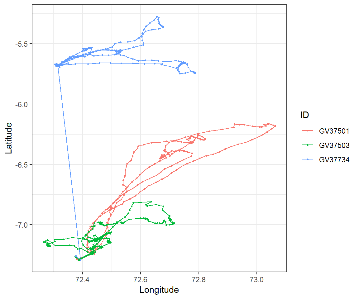
Look at the raw tracks:

Code
ggplot2::ggplot(gps_merged, ggplot2::aes(x = lon, y = lat, colour = ID)) +
  ggplot2::geom_path() +   # joins the fixes in time order
  ggplot2::geom_point(size = 0.5) +
  ggplot2::labs(x = "Longitude", y = "Latitude") +
  ggplot2::theme_bw()

Some fixes for GV37734 look wrong: they are far away from the rest of the track. Before dealing with them, check for duplicates and missing data (Week 1).

Duplicates and missing fixes

Code
sum(duplicated(gps_merged))   # duplicated rows
[1] 0
Code
colSums(is.na(gps_merged))    # missing values in each column
           ID     date_time           lon           lat    Population 
            0             0             0             0             0 
BreedingStage   deploy_time      nest_lon      nest_lat 
            0             0             0             0 

There are no duplicated rows and no missing values in these data (if there were, dplyr::distinct() would remove the duplicates). A few random missing fixes are not a problem, but many consecutive missing fixes are not random. For example, dense forest canopy blocks GPS signals, which biases the data against forest habitats.

Code
gps_merged <- gps_merged %>%
  dplyr::distinct()

Movement metrics

To find impossible fixes, calculate for each fix (within each bird):

  • the distance from the previous fix,
  • the time since the previous fix,
  • the speed (distance / time),
  • the net displacement: the distance from the first fix (the nest).

geosphere::distHaversine() calculates the distance in metres between two sets of longitude/latitude points, allowing for the curvature of the Earth. dplyr::lag() gives the previous value, and dplyr::first() the first value.

Code
gps_metrics <- gps_merged %>%
  dplyr::group_by(ID) %>%                                       # calculate within each bird
  dplyr::mutate(
    dist_m     = geosphere::distHaversine(cbind(lon, lat), cbind(dplyr::lag(lon), dplyr::lag(lat))),
    time_s     = as.numeric(difftime(date_time, dplyr::lag(date_time), units = "secs")),
    speed_ms   = dist_m / time_s,                               # metres per second
    netdisp_km = geosphere::distHaversine(cbind(lon, lat), cbind(dplyr::first(lon), dplyr::first(lat))) / 1000) %>%
  dplyr::ungroup()

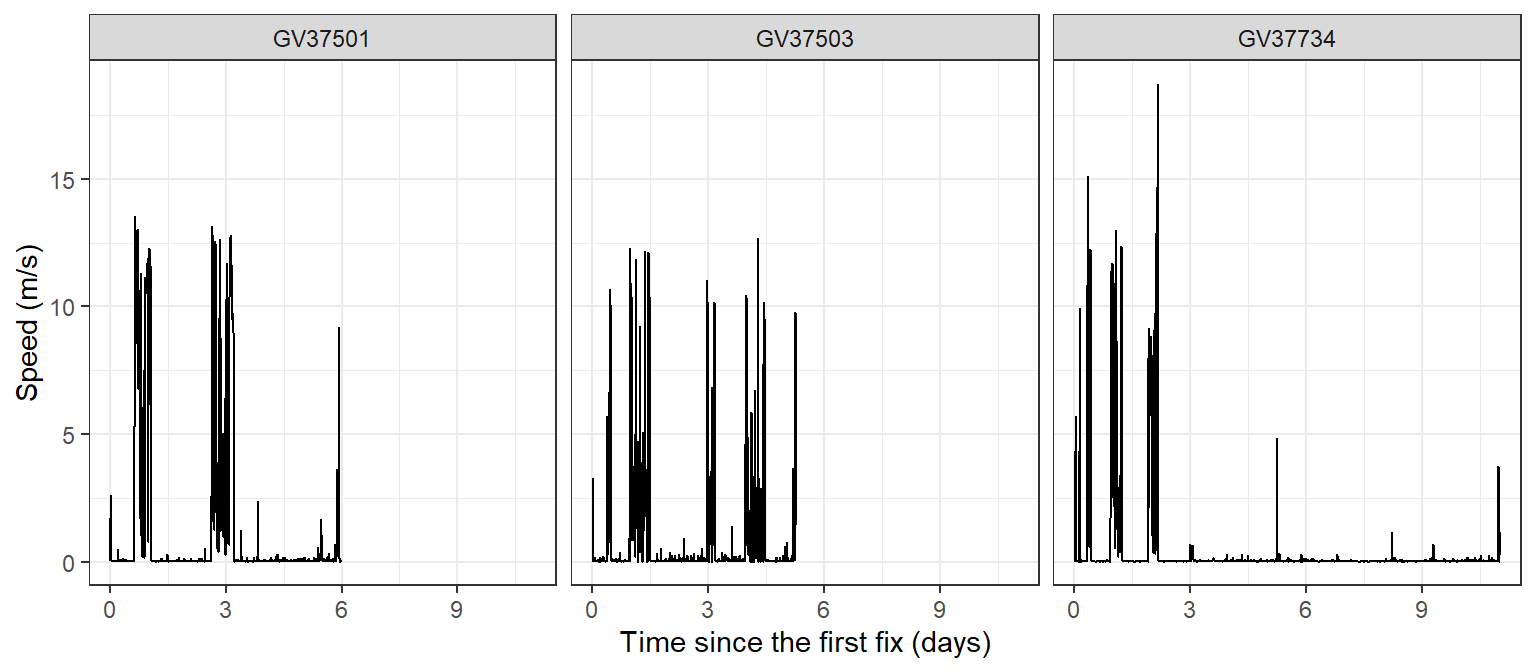
summary(gps_metrics$speed_ms)
    Min.  1st Qu.   Median     Mean  3rd Qu.     Max.      NAs 
 0.00000  0.01305  0.02700  0.67629  0.07005 18.70463        3 

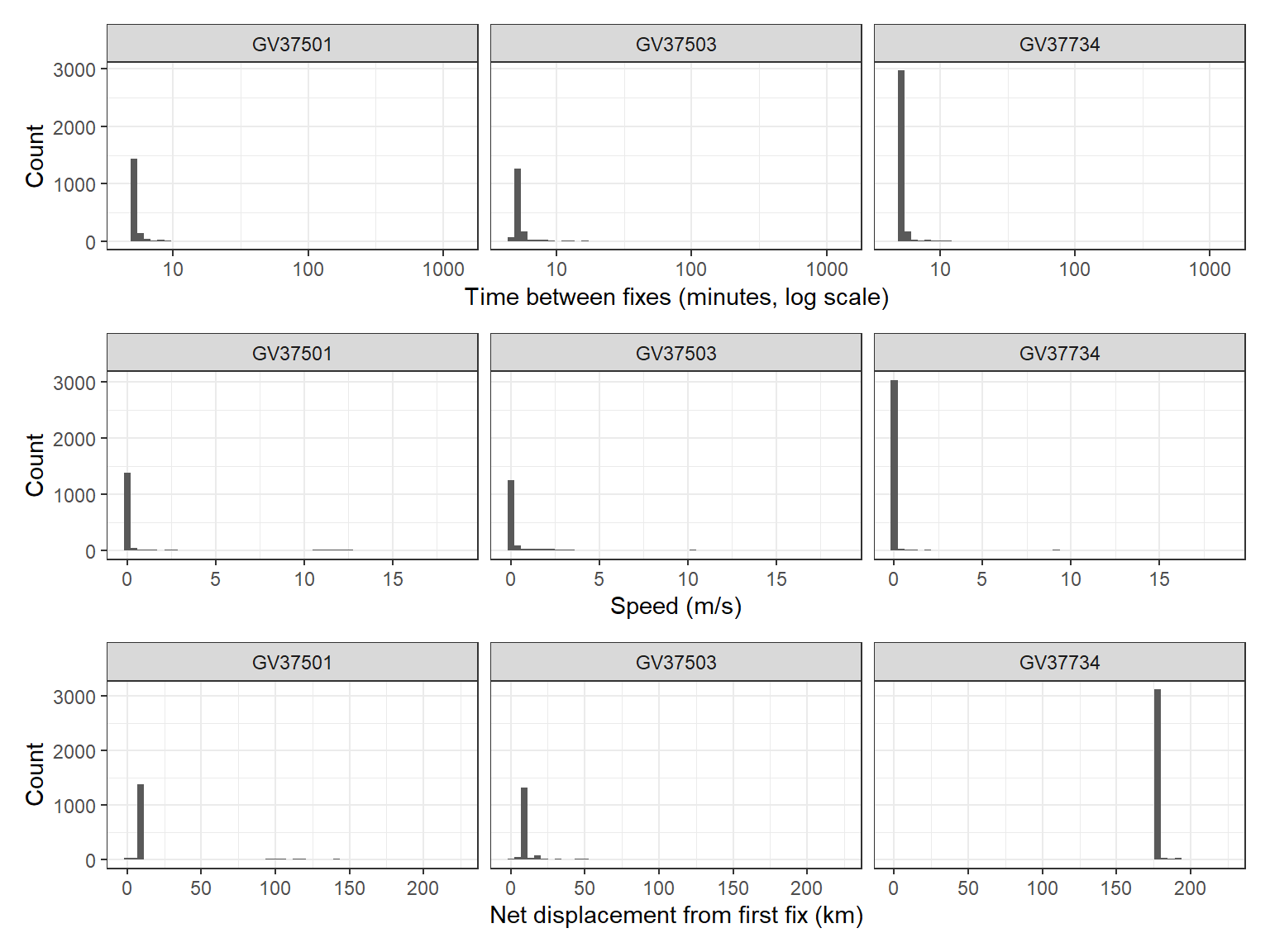
Plot the distributions of these metrics to spot errors:

Code
time_plot <- ggplot2::ggplot(gps_metrics, ggplot2::aes(x = time_s / 60)) +
  ggplot2::geom_histogram(bins = 50) +
  ggplot2::scale_x_log10() +                       # log scale: most gaps are short
  ggplot2::labs(x = "Time between fixes (minutes, log scale)", y = "Count") +
  ggplot2::facet_wrap(~ ID) +
  ggplot2::theme_bw()

speed_plot <- ggplot2::ggplot(gps_metrics, ggplot2::aes(x = speed_ms)) +
  ggplot2::geom_histogram(bins = 50) +
  ggplot2::labs(x = "Speed (m/s)", y = "Count") +
  ggplot2::facet_wrap(~ ID) +
  ggplot2::theme_bw()

disp_plot <- ggplot2::ggplot(gps_metrics, ggplot2::aes(x = netdisp_km)) +
  ggplot2::geom_histogram(bins = 50) +
  ggplot2::labs(x = "Net displacement from first fix (km)", y = "Count") +
  ggplot2::facet_wrap(~ ID) +
  ggplot2::theme_bw()

time_plot / speed_plot / disp_plot

Filter out errors

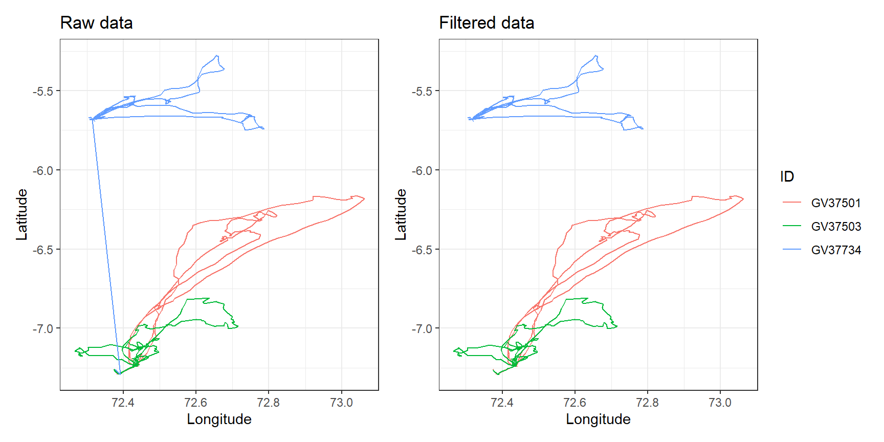
Choose thresholds from the biology of your species (and the literature), then filter:

  • Deployment period: remove the first 30 minutes after the tag was attached, when the bird may behave unnaturally after handling.
  • Speed: red-footed boobies rarely fly faster than about 20 m/s, so faster “movements” are GPS errors.
  • Net displacement: these birds were rearing chicks and returning to the nest, so fixes more than 300 km away are errors.

If your GPS data have a dilution of precision (DOP) column, you can also remove fixes with poor precision (e.g. DOP > 8).

Code
gps_clean <- gps_metrics %>%
  dplyr::filter(date_time > deploy_time + lubridate::minutes(30), # after the first 30 min
                is.na(speed_ms) | speed_ms < 20,                 # keep the first fix (no speed) and realistic speeds
                netdisp_km <= 300)                               # within 300 km of the start

# How many fixes were removed for each bird?
dplyr::left_join(dplyr::count(gps_metrics, ID, name = "before"),
                 dplyr::count(gps_clean, ID, name = "after"),
                 by = "ID")
# A tibble: 3 × 3
  ID      before after
  <chr>    <int> <int>
1 GV37501   1725  1609
2 GV37503   1646  1364
3 GV37734   3279  3069
Code
raw_plot <- ggplot2::ggplot(gps_metrics, ggplot2::aes(x = lon, y = lat, colour = ID)) +
  ggplot2::geom_path() +
  ggplot2::labs(title = "Raw data", x = "Longitude", y = "Latitude") +
  ggplot2::theme_bw()

clean_plot <- ggplot2::ggplot(gps_clean, ggplot2::aes(x = lon, y = lat, colour = ID)) +
  ggplot2::geom_path() +
  ggplot2::labs(title = "Filtered data", x = "Longitude", y = "Latitude") +
  ggplot2::theme_bw()

raw_plot + clean_plot + patchwork::plot_layout(guides = "collect") # one shared legend

NoteCoordinate reference systems

Longitude and latitude are in degrees (CRS code EPSG:4326). geosphere handles these directly. If you combine tracks with other maps or rasters (e.g. habitat or sea surface temperature), make sure every layer uses the same coordinate reference system, and use a projected CRS in metres for area calculations such as home ranges. See the optional spatial data tutorial and the EPSG database.

Plot the clean data

Other tracking data

Other technologies need different cleaning steps:

  • Argos tags: each location has a location class (accuracy category) instead of a DOP. Error estimates differ among classes, and tracks are often processed with state-space models.
  • Acoustic telemetry: sound signals are easily corrupted, so false detections occur. Detections of tag IDs that are not in your study are easy to remove, but false detections of real tag IDs are harder to spot. Most studies use speed filters or summarise detections over longer time periods.

Analysing movement data

Movement analysis is beyond this unit, because it needs models that handle autocorrelated, multidimensional (x, y, time) and irregularly sampled data. Some possibilities:

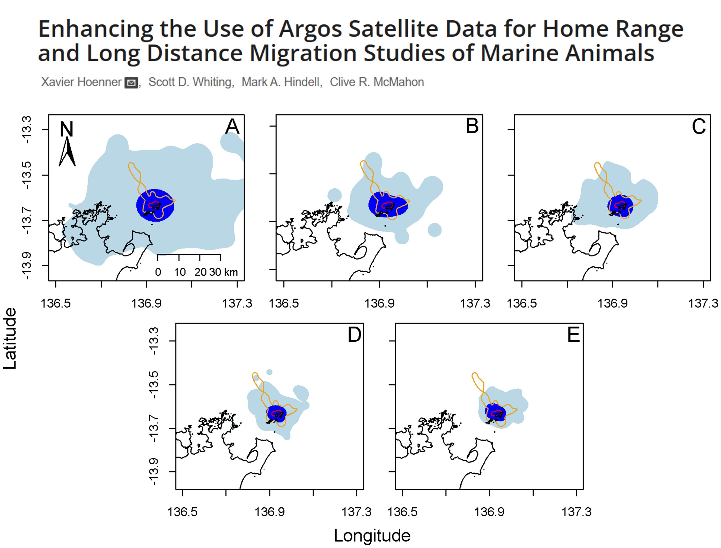
  • Home range / space use: minimum convex polygons (MCP), kernel density estimates (KDE) and autocorrelated KDE (AKDE).
Method Complexity Data needed Gives intensity of use? Best for
MCP Very simple Low (≥ 30 points) No Coarse, presence-only questions
KDE Moderate Moderate (≥ 50 points) Yes Core areas
AKDE High High (≥ 100 points) Yes Rigorous inference from intensive GPS data
ImportantHome range or space use?

A home range is “that area traversed by an individual in its normal activities of food gathering, mating and caring for young” (Burt, 1943). Tracking data alone cannot show whether an area is used for all these activities, and an animal tracked for one season may use a completely different area in another. The safest term is space use, interpreted in the context of the study design (e.g. one week vs several months of tracking).

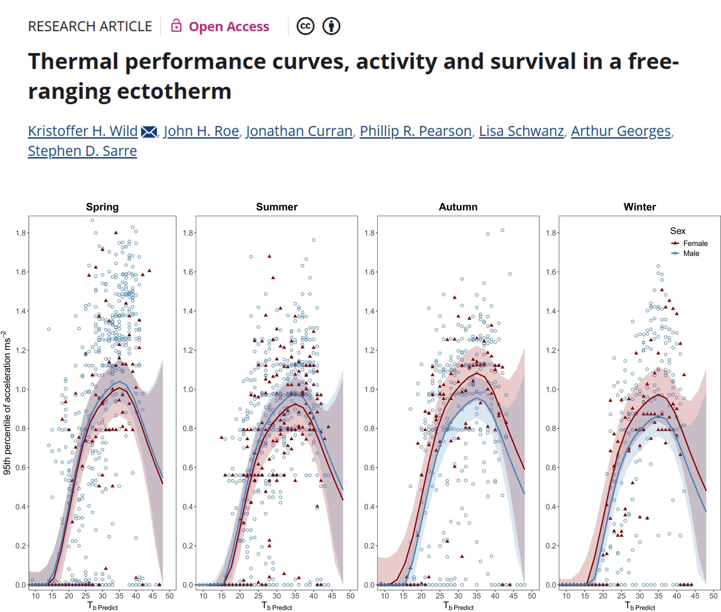
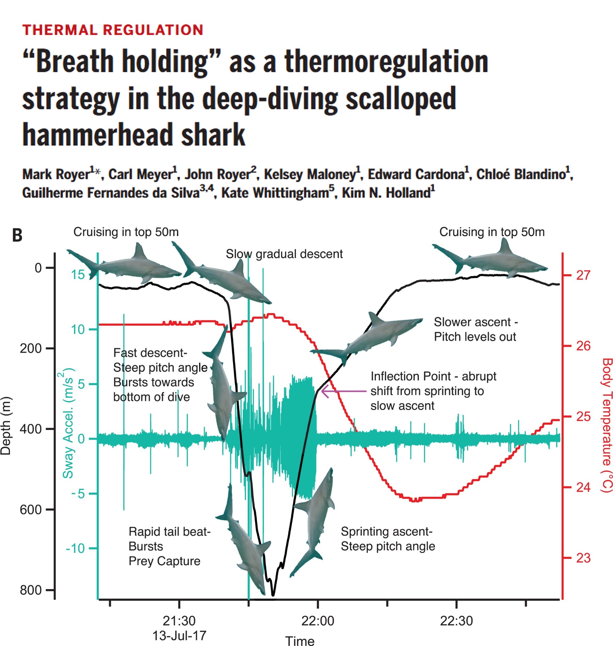
  • Behavioural states: high-resolution movement and accelerometer data can separate resting, foraging and travelling using methods such as hidden Markov models.

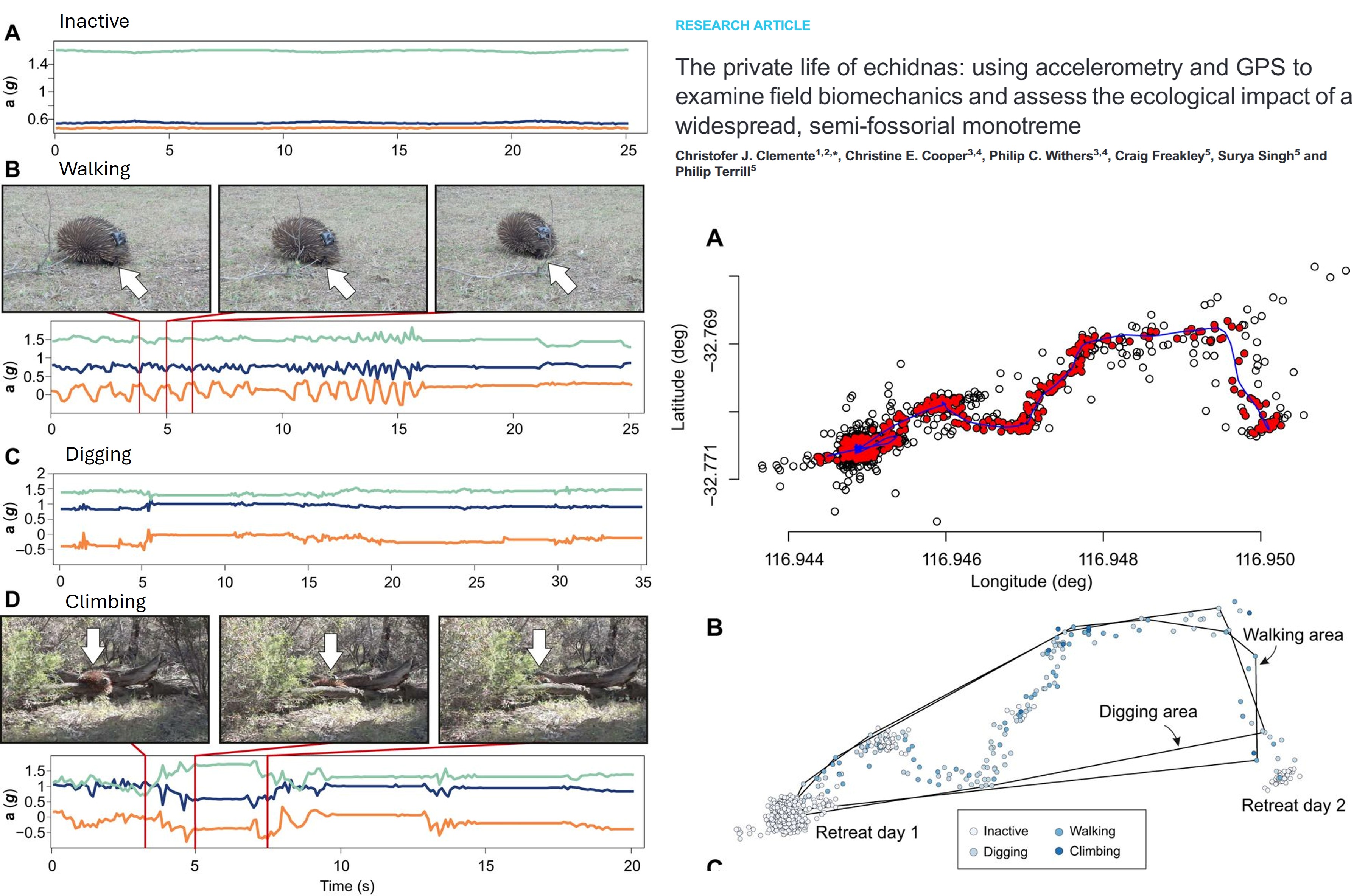
Classifying echidna behaviour from accelerometer traces (Clemente et al., 2016).
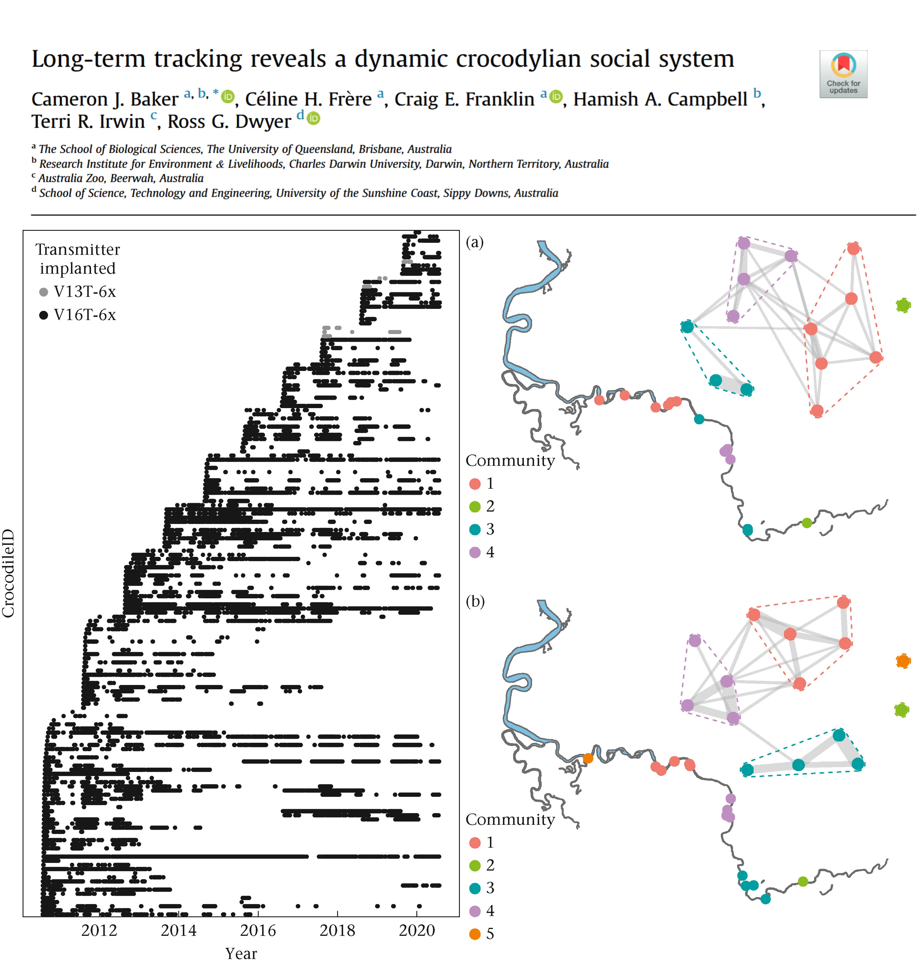
  • Social networks: when and where tracked animals meet can be used to build social networks.
  • Disease spread: movement data help predict how diseases spread through populations, as seen for COVID-19.

Additional resources