7  Linear and Multiple Regression

Week 7: Relationships between a response and one or more numeric predictors

In Week 5 you compared groups. This week the predictor is a number (latitude, temperature, chlorophyll) and we ask how the response changes as that number changes. You will fit a simple linear regression (one predictor) and then a multiple regression (several predictors). Workshop materials are available in the GitHub repository ECS200.

TipLearning outcomes

By the end of this workshop you should be able to:

  1. Explain what the intercept, slope and R2 of a regression mean.
  2. Use diagnostic plots to check linearity, equal variance, normality and influential points.
  3. Recognise collinearity between predictors and decide what to do about it.
  4. Fit, visualise and write up simple and multiple regression models in R.

Before we start

pie_crab.csv coralreefdata.csv

We use one new package, ggeffects, to plot what a model predicts.

Code
# Week 7 workshop - Linear and multiple regression
# Written by Nicholas Wu, 1234578, 15/04/2027

# install.packages("ggeffects")  # run once in the console if needed

library(tidyverse)   # data import, wrangling and plotting
library(performance) # checking model assumptions
library(see)         # draws the plots for performance
library(ggeffects)   # predictions from models for plotting

# setwd("C:/Users/YOUR-NAME/Documents/ECS200")

Part A: Simple linear regression

Question: Are fiddler crabs bigger at higher latitudes (Bergmann’s rule)?

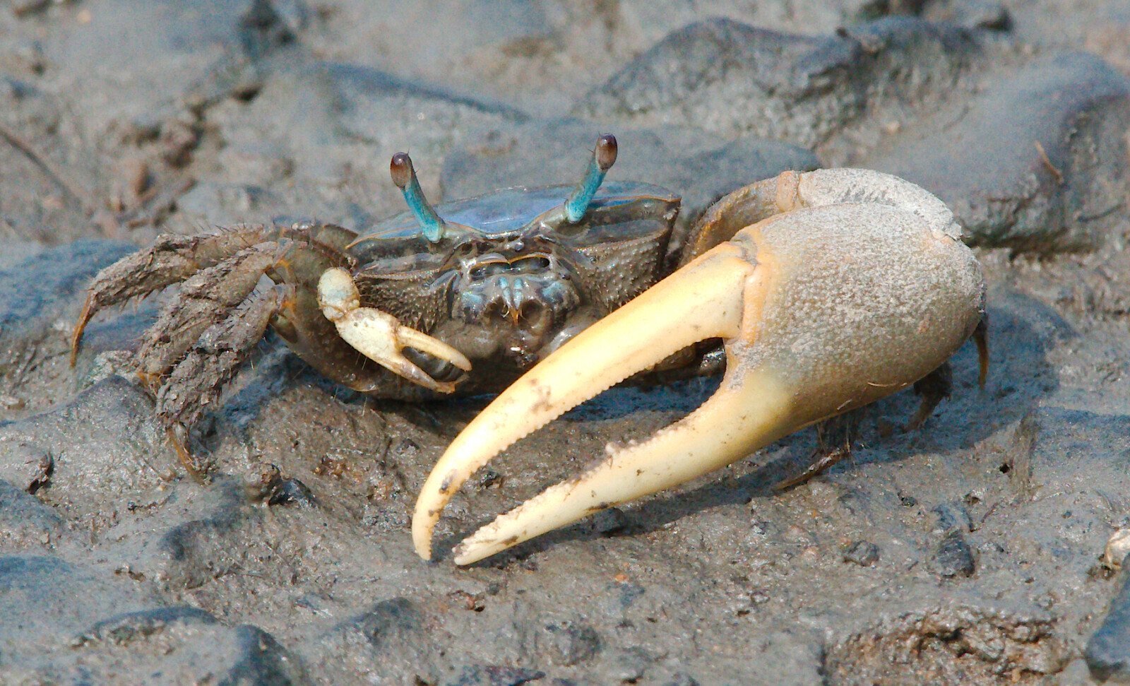
Bergmann’s rule predicts that individuals of a species are larger in colder places, which usually means at higher latitudes. In summer 2016, researchers measured the carapace width of adult male Atlantic marsh fiddler crabs (Minuca pugnax) at 13 salt marshes spanning more than 12 degrees of latitude, from Florida to Massachusetts (Johnson, 2019). The data come from the lterdatasampler collection.

Atlantic marsh fiddler crab (Minuca pugnax).
Code
crab_data <- readr::read_csv("data/pie_crab.csv")

dplyr::glimpse(crab_data)
Rows: 392
Columns: 9
$ date          <date> 2016-07-24, 2016-07-24, 2016-07-24, 2016-07-24, 2016-07…
$ latitude      <dbl> 30, 30, 30, 30, 30, 30, 30, 30, 30, 30, 30, 30, 30, 30, …
$ site          <chr> "GTM", "GTM", "GTM", "GTM", "GTM", "GTM", "GTM", "GTM", …
$ size          <dbl> 12.43, 14.18, 14.52, 12.94, 12.45, 12.99, 10.32, 11.19, …
$ air_temp      <dbl> 21.792, 21.792, 21.792, 21.792, 21.792, 21.792, 21.792, …
$ air_temp_sd   <dbl> 6.391, 6.391, 6.391, 6.391, 6.391, 6.391, 6.391, 6.391, …
$ water_temp    <dbl> 24.502, 24.502, 24.502, 24.502, 24.502, 24.502, 24.502, …
$ water_temp_sd <dbl> 6.121, 6.121, 6.121, 6.121, 6.121, 6.121, 6.121, 6.121, …
$ name          <chr> "Guana Tolomoto Matanzas NERR", "Guana Tolomoto Matanzas…

The columns we need are size (carapace width, mm) and latitude (degrees north).

1. Background

A simple linear regression fits the straight line that best describes how a numeric response (y) changes with a numeric predictor (x):

\[ y_i = \beta_0 + \beta_1 x_i + \varepsilon_i \]

  • \(\beta_0\) is the intercept: the predicted y when x = 0.
  • \(\beta_1\) is the slope: how much y changes, on average, for every one-unit increase in x. This is usually the number your research question is about.
  • \(\varepsilon_i\) is the residual: the vertical distance between each point and the line. Residuals are assumed to be normally distributed with constant spread.

R finds the line that makes the sum of the squared residuals as small as possible (least squares). The null hypothesis is that the slope is zero (no relationship).

A straight line is only a good summary if the relationship really is straight. In the app below, choose a pattern and compare the diagnostic plots with the ideal: a flat, patternless cloud in the residuals plot and points along the line in the Q-Q plot.

App: is a straight line a good fit?

2. Visualise

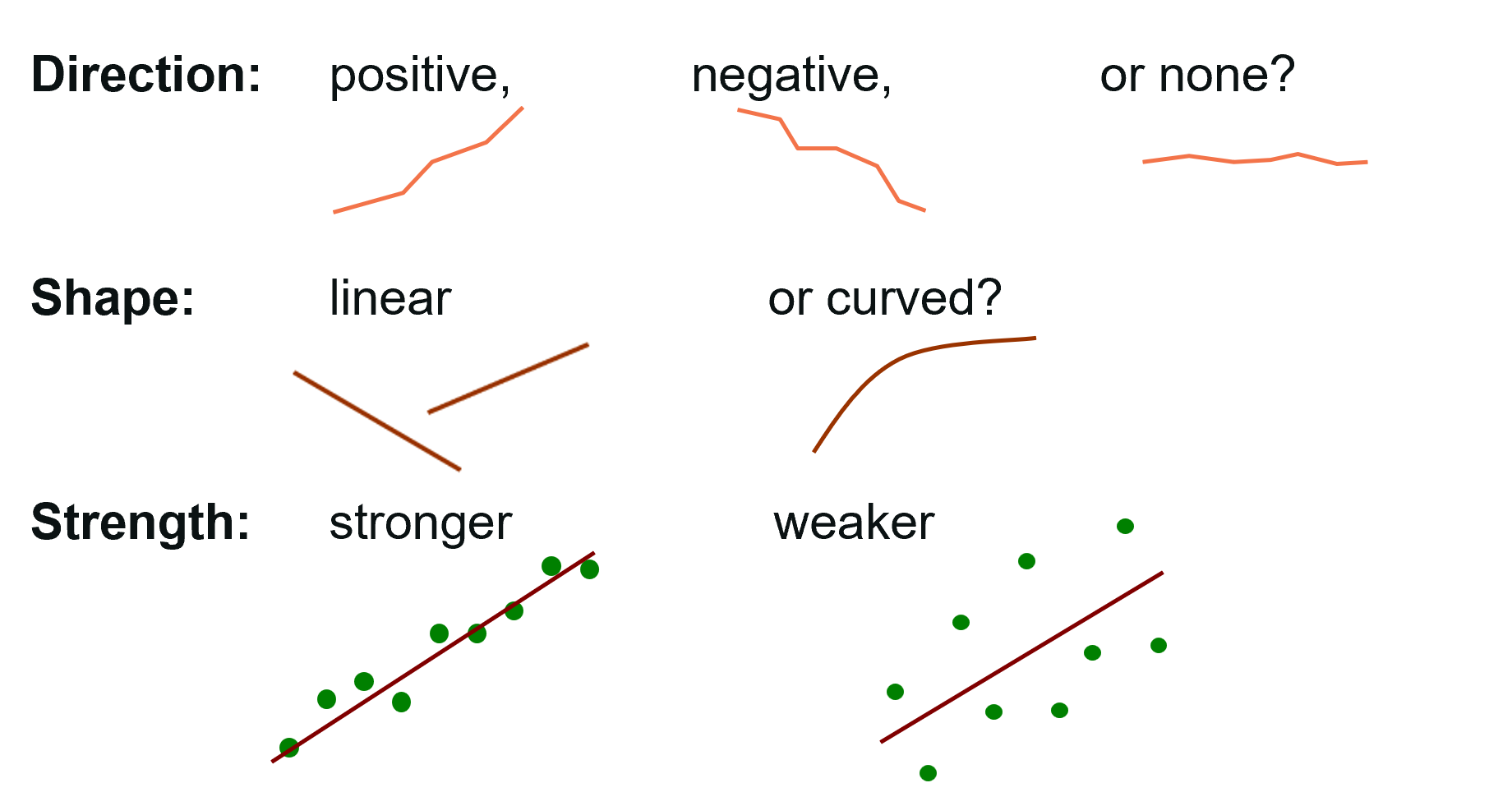
Always plot the data before fitting a model. Describe the direction (positive or negative), form (linear or curved), strength (tight or scattered) and any unusual points.

What to describe when looking at a scatterplot.
Code
ggplot2::ggplot(crab_data, ggplot2::aes(x = latitude, y = size)) +
  ggplot2::geom_point(alpha = 0.4) +
  ggplot2::labs(x = "Latitude (°N)", y = "Carapace width (mm)") +
  ggplot2::theme_classic()

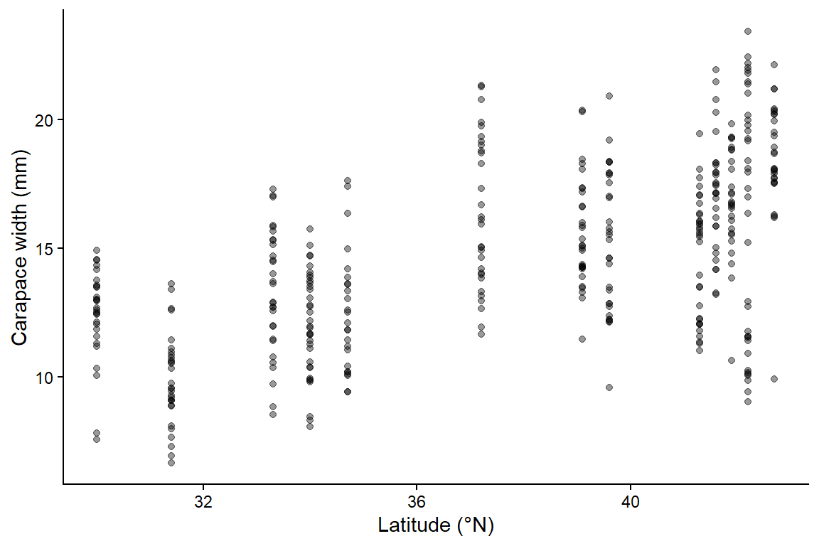
The relationship is positive (crabs are wider further north), roughly linear, of moderate strength, and there are no obvious errors. Notice that the points form 13 vertical stripes: every crab from the same marsh shares the same latitude. Keep that in mind for the independence assumption below.

3. Check assumptions

Fit the model first, then check the residuals with performance::check_model().

Code
# size explained by latitude
crab_lm <- lm(size ~ latitude, data = crab_data)
Code
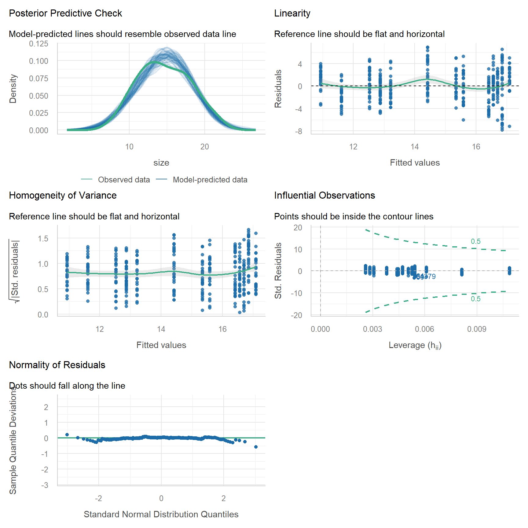
performance::check_model(crab_lm)

Each panel has a subtitle that describes what you want to see:

Panel Checks What you want to see Here
Posterior predictive check Overall fit Model-predicted lines (blue) resemble the data (green) ✅
Linearity Straight-line relationship Flat, horizontal reference line ✅
Homogeneity of variance Equal spread of residuals Flat, horizontal reference line ✅ Roughly flat
Influential observations Single points controlling the fit All points inside the contour lines ✅
Normality of residuals Normal residuals Dots fall along the line ✅ Slight wobble in the tails, acceptable with n = 392

The plots cannot check independence. That comes from the study design: 392 crabs were measured, but they come from only 13 marshes, and crabs from the same marsh share the same environment. This means we have less independent information than 392 data points suggest, and the p-value will be too small. We will handle this properly with a mixed-effects model in Week 12. For now we note it as a caveat.

Influential points deserve a closer look. Use the app to see how a single point can change the regression line, depending on where it sits.

App: leverage and influential points

Leverage measures how unusual a point’s x value is. Cook’s distance combines leverage with the size of the residual. A point is only a problem when it is both unusual in x and far from the line. Never delete a point just because it is influential. Check whether it is a data entry error (Week 1) and, if it is real, report the results with and without it.

What you see Problem What to do instead
Curved pattern in the scatterplot or a U-shape in the residuals Relationship is not linear Transform x and/or y (e.g. log, see the Assessment), or add a curved term y ~ x + I(x^2). For wiggly relationships, use a generalised additive model (Pedersen et al., 2019)
Residual spread increases with fitted values (fan shape) Unequal variance Log-transform y, or use a GLM (Weeks 8 and 11)
Observations grouped by site, individual or time Not independent Mixed-effects model (Week 12)
Response is a count, a proportion or yes/no Residuals cannot be normal GLM (Weeks 8 and 11)
Predictor measured with large error Slope is biased towards zero Discuss as a caveat. Better measurements are the real fix

4. Model

Code
# Coefficients, standard errors, t values, p-values and R-squared
summary(crab_lm)

Call:
lm(formula = size ~ latitude, data = crab_data)

Residuals:
    Min      1Q  Median      3Q     Max 
-7.8376 -1.8797  0.1144  1.9484  6.9280 

Coefficients:
            Estimate Std. Error t value Pr(>|t|)    
(Intercept) -3.62442    1.27405  -2.845  0.00468 ** 
latitude     0.48512    0.03359  14.441  < 2e-16 ***
---
Signif. codes:  0 '***' 0.001 '**' 0.01 '*' 0.05 '.' 0.1 ' ' 1

Residual standard error: 2.832 on 390 degrees of freedom
Multiple R-squared:  0.3484,    Adjusted R-squared:  0.3467 
F-statistic: 208.5 on 1 and 390 DF,  p-value: < 2.2e-16
Code
# 95% confidence intervals for the intercept and slope
confint(crab_lm)
                 2.5 %    97.5 %
(Intercept) -6.1292889 -1.119554
latitude     0.4190732  0.551165

The output gives everything you need:

  • Residuals: a summary of the residuals. The median should be close to 0, and the minimum and maximum (and 1Q and 3Q) roughly the same distance from it.
  • Coefficients: one row for the intercept and one for the slope.
    • Estimate: (Intercept) is the predicted width at latitude 0; latitude is the slope, the change in width (mm) per degree of latitude. A positive slope means width increases with latitude.
    • Std. Error: the uncertainty in each estimate.
    • t value: the estimate divided by its standard error.
    • Pr(>|t|): the p-value for the null hypothesis that the coefficient is 0 (for the slope: no relationship).
  • Residual standard error: the typical distance of a crab from the fitted line (mm), with its degrees of freedom (number of crabs − 2).
  • Multiple R-squared: the proportion of variation in width explained by latitude. Adjusted R-squared is slightly lower because it penalises extra predictors; it matters more in multiple regression.
  • F-statistic ... on 1 and ... DF, p-value: compares this model with a model that has no predictor. With one predictor its p-value equals the slope’s p-value.
  • confint(): the 95% confidence intervals (2.5 % to 97.5 %) for the intercept and slope. If the slope’s CI does not include 0, the relationship is significant at α = 0.05.

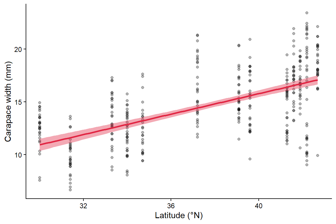
Add the fitted line and its 95% confidence band to the scatterplot. geom_smooth(method = "lm") fits the same model as lm(size ~ latitude).

Code
ggplot2::ggplot(crab_data, ggplot2::aes(x = latitude, y = size)) +
  ggplot2::geom_point(alpha = 0.3) +
  ggplot2::geom_smooth(method = "lm", colour = "#e12744", fill = "#e12744") + # line + 95% CI
  ggplot2::labs(x = "Latitude (°N)", y = "Carapace width (mm)") +
  ggplot2::theme_classic()

5. Interpret

The fitted model is:

\[ \widehat{\text{width}} = -3.62 + 0.485 \times \text{latitude} \]

  • Slope (0.485): carapace width increases by about 0.49 mm for every degree further north (95% CI 0.42–0.55 mm). Across the 12 degrees sampled, that is about 5.8 mm.
  • Intercept (-3.62): the predicted width at latitude 0 (the equator). This is outside the range of the data and a negative width is impossible, so the intercept has no biological meaning here. That is common, and fine.
  • R2 (0.35): latitude explains 35% of the variation in carapace width. The rest is variation among individual crabs.
  • F-test at the bottom: compares this model with a model that has no predictor. With one predictor its p-value equals the slope’s p-value.

Methods sentence: The relationship between carapace width and latitude was analysed with a simple linear regression using the lm() function in R. Model assumptions were checked with diagnostic plots using the performance package. Significance was set at α = 0.05.

Results sentence:

Consistent with Bergmann’s rule, fiddler crabs were larger at higher latitudes. Carapace width increased by 0.49 mm per degree of latitude (95% CI 0.42–0.55; F1,390 = 208.5, p < 0.001, R2 = 0.35; Fig. 1). Because crabs were sampled from only 13 marshes, this p-value is likely too small (see Week 12).

Part B: Multiple regression

Question: Which environmental factors are associated with coral reef diversity?

This simulated dataset describes reef health (the Shannon diversity index of the coral community, Week 4) at 72 reef sites, together with five potential predictors:

  • sst: sea surface temperature at the time of the visit (°C)
  • pH: surface water pH
  • chlorophyll: chlorophyll-a concentration (mg/m3), a proxy for nutrient run-off and poor water clarity
  • distance_from_land: distance from the coast (km)
  • fishing_allowed: whether commercial fishing is allowed (Yes/No)

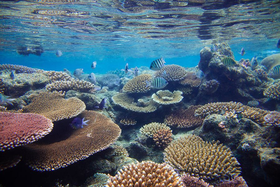
The Great Barrier Reef.
Code
reef_data <- readr::read_csv("data/coralreefdata.csv") %>%
  dplyr::mutate(fishing_allowed = factor(fishing_allowed)) # categorical predictor

dplyr::glimpse(reef_data)
Rows: 72
Columns: 6
$ shannon            <dbl> 2.401169, 3.300000, 2.975029, 2.006727, 2.831517, 3…
$ sst                <dbl> 28.40798, 27.20761, 27.06746, 28.99881, 27.06975, 2…
$ pH                 <dbl> 8.096462, 8.093622, 8.111877, 8.094532, 8.100962, 8…
$ chlorophyll        <dbl> 0.1499800, 0.1815619, 0.2310620, 0.4149387, 0.11594…
$ distance_from_land <dbl> 78.53486, 70.32110, 62.20095, 37.52461, 83.42137, 7…
$ fishing_allowed    <fct> Yes, No, Yes, No, Yes, No, No, Yes, No, No, Yes, Ye…

1. Background

Multiple regression adds more predictors to the same equation:

\[ y_i = \beta_0 + \beta_1 x_{1i} + \beta_2 x_{2i} + \dots + \varepsilon_i \]

Each slope is now a partial effect: the change in y for a one-unit change in that predictor while all other predictors are held constant. This lets you separate the effects of predictors that would otherwise be tangled together, for example temperature and fishing.

Predictors can be numbers or categories. For a categorical predictor such as fishing_allowed, the coefficient is the difference in mean y between that category and the reference category (here “No”).

Collinearity is the big trap. When two predictors are strongly correlated with each other (e.g. chlorophyll is high close to land and low far from land), the model cannot tell which one is responsible. The estimates become unstable: standard errors grow, slopes can flip sign, and neither predictor may look significant even though together they explain a lot (Dormann et al., 2013). The variance inflation factor (VIF) measures this. VIF < 5 is fine, 5–10 is worrying and > 10 is serious.

App: what collinearity does to your estimates

2. Visualise

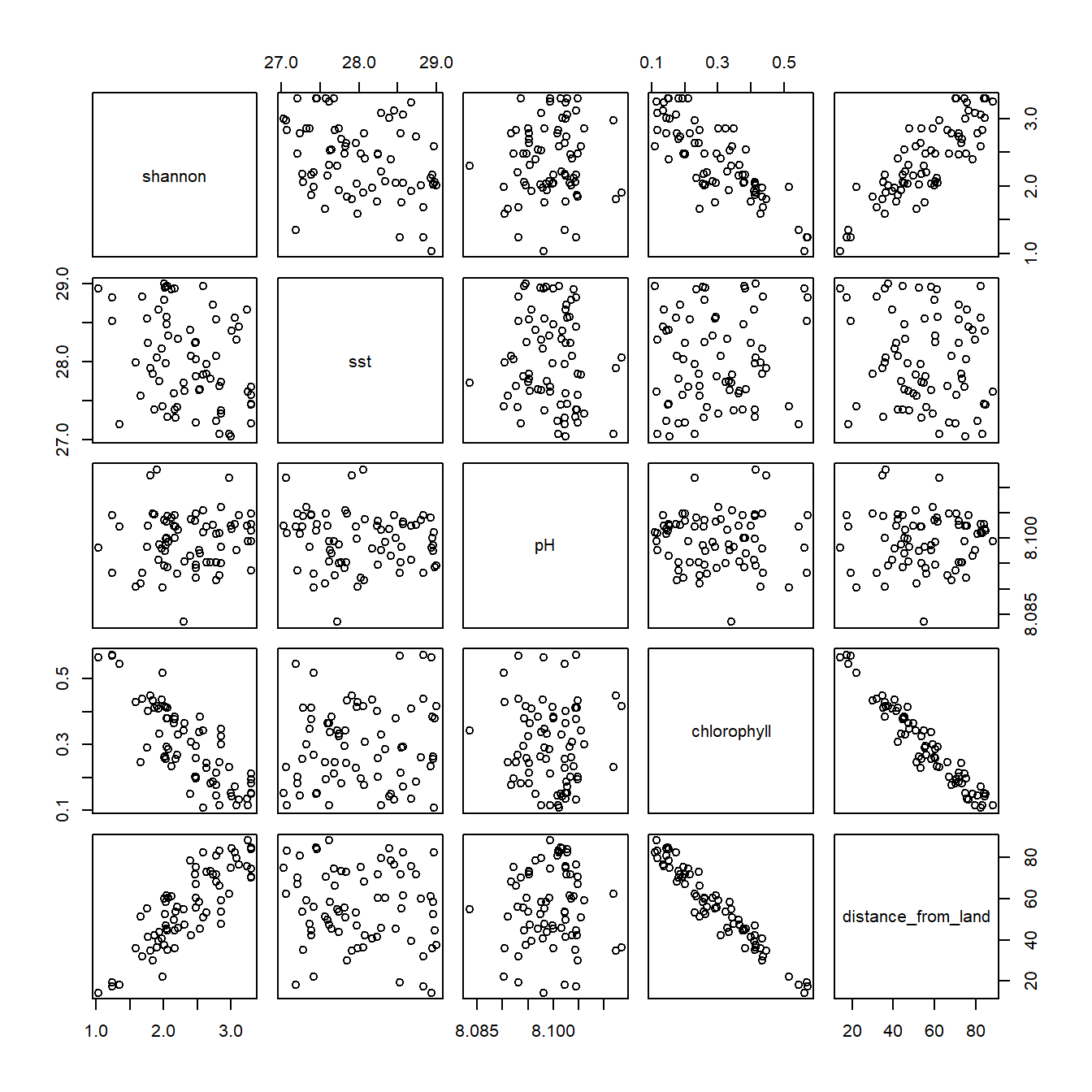
With several predictors, look at every pair of variables at once. pairs() draws a scatterplot for each pair, and cor() gives the correlation coefficients.

Code
# Scatterplot of every pair of numeric variables
reef_data %>%
  dplyr::select(shannon, sst, pH, chlorophyll, distance_from_land) %>%
  pairs()

Code
# Correlation matrix (rounded to 2 decimal places)
reef_data %>%
  dplyr::select(shannon, sst, pH, chlorophyll, distance_from_land) %>%
  cor() %>%
  round(2)
                   shannon   sst    pH chlorophyll distance_from_land
shannon               1.00 -0.33  0.08       -0.81               0.84
sst                  -0.33  1.00 -0.09        0.12              -0.14
pH                    0.08 -0.09  1.00       -0.05               0.03
chlorophyll          -0.81  0.12 -0.05        1.00              -0.97
distance_from_land    0.84 -0.14  0.03       -0.97               1.00
Code
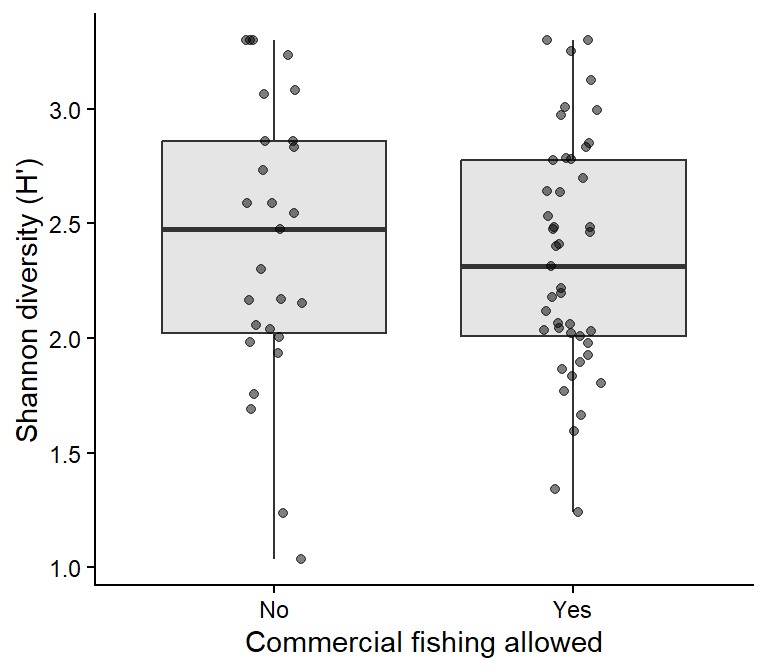
# The categorical predictor
ggplot2::ggplot(reef_data, ggplot2::aes(x = fishing_allowed, y = shannon)) +
  ggplot2::geom_boxplot(outlier.shape = NA, fill = "grey90") +
  ggplot2::geom_jitter(width = 0.1, alpha = 0.5) +
  ggplot2::labs(x = "Commercial fishing allowed", y = "Shannon diversity (H')") +
  ggplot2::theme_classic()

What do we see?

  • Diversity decreases strongly with chlorophyll and increases with distance from land.
  • Chlorophyll and distance from land are almost perfectly correlated (r = −0.97). This is a collinearity warning.
  • The relationships look linear and diversity seems lower where fishing is allowed.

3. Check assumptions

Fit the full model with all five predictors and check it, including collinearity.

Code
reef_lm_full <- lm(shannon ~ sst + pH + chlorophyll + distance_from_land + fishing_allowed,
                   data = reef_data)

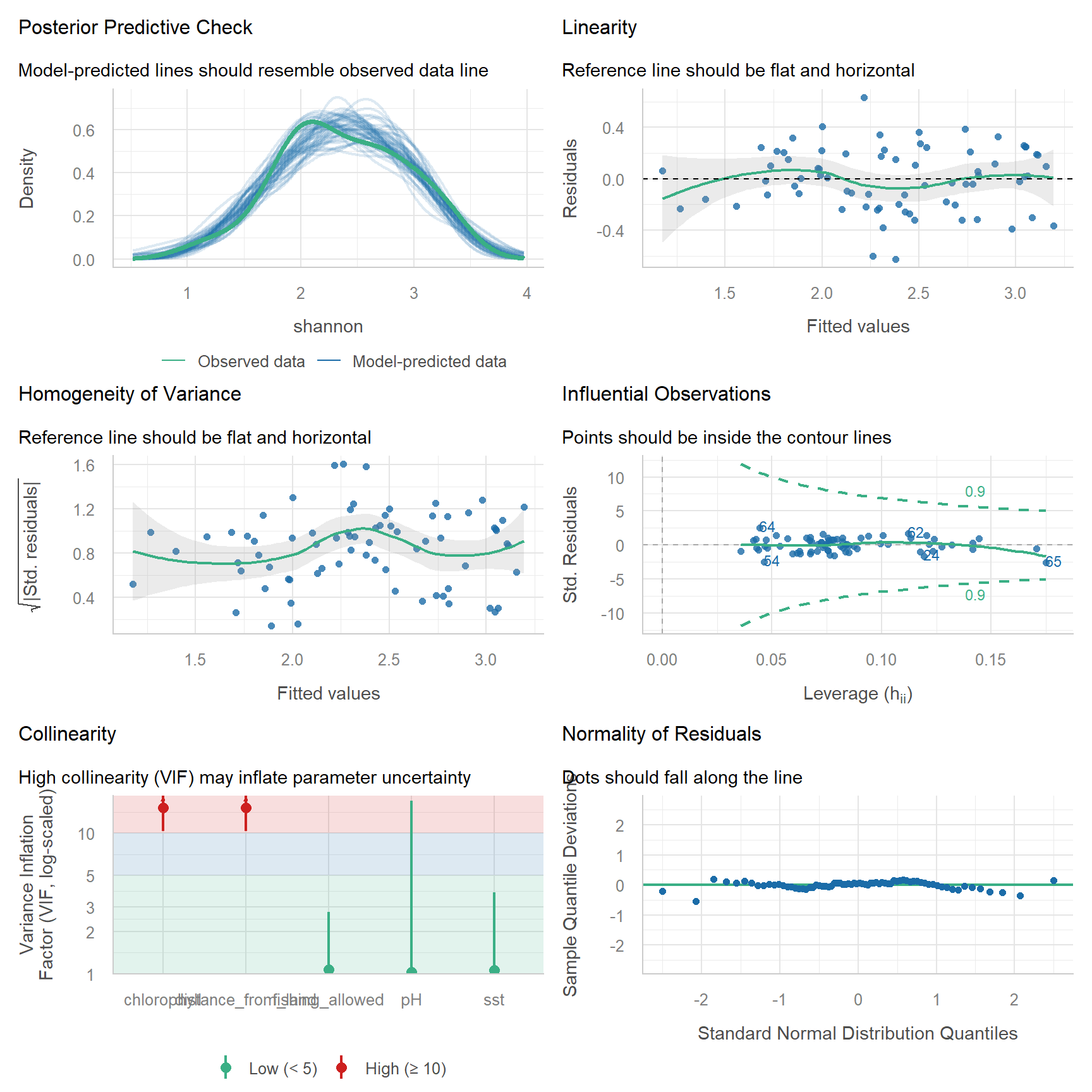
performance::check_model(reef_lm_full)

Code
# Variance inflation factors
performance::check_collinearity(reef_lm_full)
# Check for Multicollinearity

Low Correlation

            Term  VIF     VIF 95% CI adj. VIF Tolerance Tolerance 95% CI
             sst 1.06 [ 1.00,  3.80]     1.03      0.94     [0.26, 1.00]
              pH 1.04 [ 1.00, 16.94]     1.02      0.97     [0.06, 1.00]
 fishing_allowed 1.07 [ 1.00,  2.77]     1.04      0.93     [0.36, 1.00]

High Correlation

               Term   VIF     VIF 95% CI adj. VIF Tolerance Tolerance 95% CI
        chlorophyll 15.22 [10.32, 22.71]     3.90      0.07     [0.04, 0.10]
 distance_from_land 15.22 [10.31, 22.70]     3.90      0.07     [0.04, 0.10]

Chlorophyll and distance from land have very high VIFs. In this full model, chlorophyll does not even look significant (try summary(reef_lm_full)), even though it is the variable most strongly correlated with diversity. That is collinearity at work.

How to fix it: keep one of the correlated predictors. Choose using biology, not p-values. Chlorophyll is the more direct measure of water quality, which is what affects corals, while distance from land is only a proxy for it. So we keep chlorophyll and remove distance.

Code
reef_lm <- lm(shannon ~ sst + pH + chlorophyll + fishing_allowed, data = reef_data)

performance::check_collinearity(reef_lm) # all VIFs now close to 1
# Check for Multicollinearity

Low Correlation

            Term  VIF    VIF 95% CI adj. VIF Tolerance Tolerance 95% CI
             sst 1.05 [1.00,  6.73]     1.02      0.95     [0.15, 1.00]
              pH 1.03 [1.00, 38.53]     1.02      0.97     [0.03, 1.00]
     chlorophyll 1.03 [1.00, 75.98]     1.01      0.97     [0.01, 1.00]
 fishing_allowed 1.07 [1.00,  3.08]     1.03      0.94     [0.32, 1.00]
Code
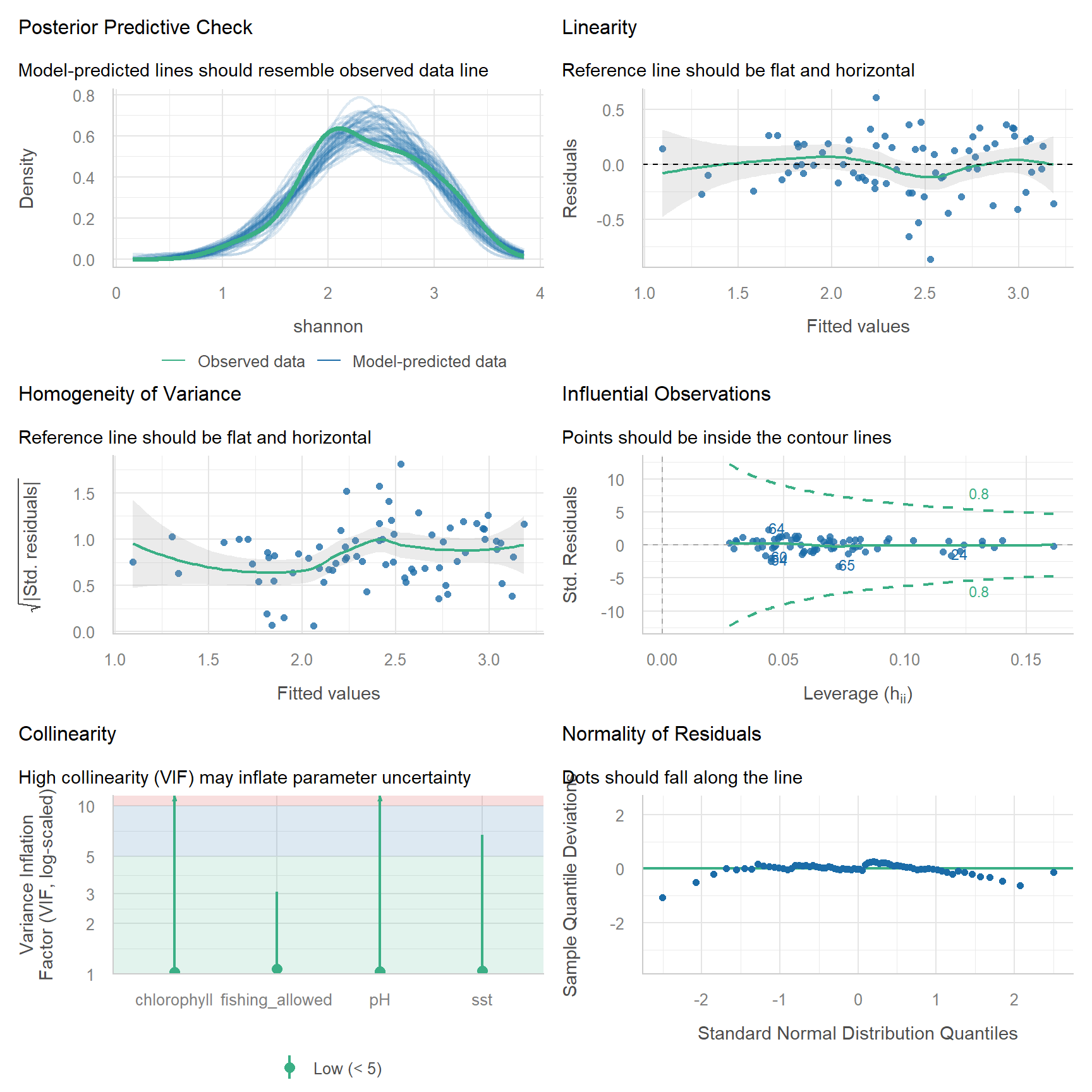
performance::check_model(reef_lm)

Assumption Check Here
Linearity Linearity panel and the pairs plot ✅
Equal variance Homogeneity panel ✅
Normal residuals Q-Q panel ✅ Close enough
No influential points Influential observations panel ✅
No collinearity VIF < 5 ✅ After removing distance from land
Independence Study design ⚠️ We assume reef sites were far enough apart to be independent
  • Too many predictors for the data. A rough rule is at least 10–20 observations per predictor. With 72 sites, 4–5 predictors is the maximum.
  • Choosing predictors by trial and error (adding and removing them until something is significant, or automated “stepwise” selection). This produces over-confident p-values. Decide which predictors to include before you analyse, based on your hypotheses, and keep non-significant predictors in the model (Harrison et al., 2018; Popovic et al., 2024).
  • Comparing the size of slopes measured in different units. A slope of −3.7 for chlorophyll and −0.26 for SST cannot be compared directly, because a 1-unit change means very different things for each.
  • Interpreting a slope outside the range of the data (extrapolation).

4. Model

Code
summary(reef_lm)

Call:
lm(formula = shannon ~ sst + pH + chlorophyll + fishing_allowed, 
    data = reef_data)

Residuals:
     Min       1Q   Median       3Q      Max 
-0.86398 -0.14961 -0.00375  0.18900  0.61316 

Coefficients:
                    Estimate Std. Error t value Pr(>|t|)    
(Intercept)        -37.22335   49.60278  -0.750  0.45562    
sst                 -0.25568    0.05674  -4.506 2.72e-05 ***
pH                   5.92832    6.10925   0.970  0.33534    
chlorophyll         -3.69597    0.27060 -13.659  < 2e-16 ***
fishing_allowedYes  -0.26429    0.06872  -3.846  0.00027 ***
---
Signif. codes:  0 '***' 0.001 '**' 0.01 '*' 0.05 '.' 0.1 ' ' 1

Residual standard error: 0.273 on 67 degrees of freedom
Multiple R-squared:  0.7699,    Adjusted R-squared:  0.7562 
F-statistic: 56.05 on 4 and 67 DF,  p-value: < 2.2e-16
Code
confint(reef_lm)
                          2.5 %     97.5 %
(Intercept)        -136.2309065 61.7842086
sst                  -0.3689359 -0.1424201
pH                   -6.2657908 18.1224398
chlorophyll          -4.2360869 -3.1558543
fishing_allowedYes   -0.4014664 -0.1271201

The output has the same parts as for the simple regression, with a few differences:

  • Coefficients: one row per predictor. Each Estimate is a partial effect: the change in diversity for a one-unit increase in that predictor, holding the others constant.
    • (Intercept): predicted diversity when every numeric predictor is 0 and fishing is “No” (the reference level). Not meaningful here (no reef has a pH of 0).
    • sst, pH, chlorophyll: the change in diversity per °C, per pH unit and per mg/m3.
    • fishing_allowedYes: the difference in mean diversity between fished (“Yes”) and unfished (“No”) reefs, at the same SST, pH and chlorophyll.
    • Std. Error, t value and Pr(>|t|): as before, one test for each predictor.
  • Residual standard error ... on ... degrees of freedom: the df is now the number of sites minus the number of coefficients (72 − 5 = 67).
  • Multiple R-squared and Adjusted R-squared: the proportion of variation explained by all predictors together. Report the adjusted R2 when comparing models with different numbers of predictors, because R2 always increases when you add one.
  • F-statistic: tests whether the predictors together explain more than a model with no predictors. It can be significant even when no single predictor is.
  • confint(): the 95% CIs for each coefficient. A CI that includes 0 means no clear effect of that predictor.

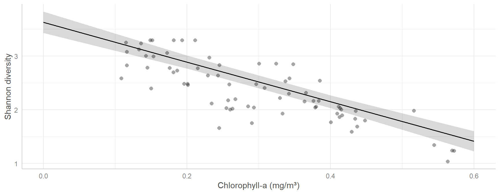
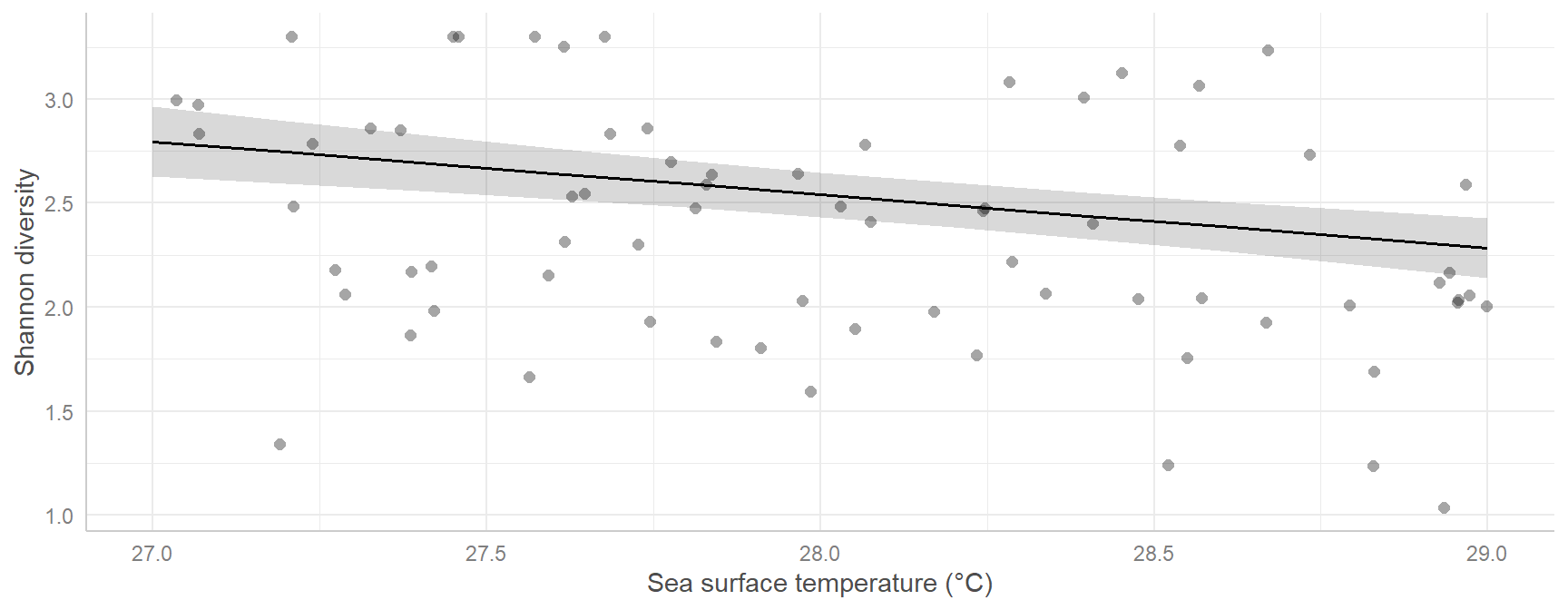
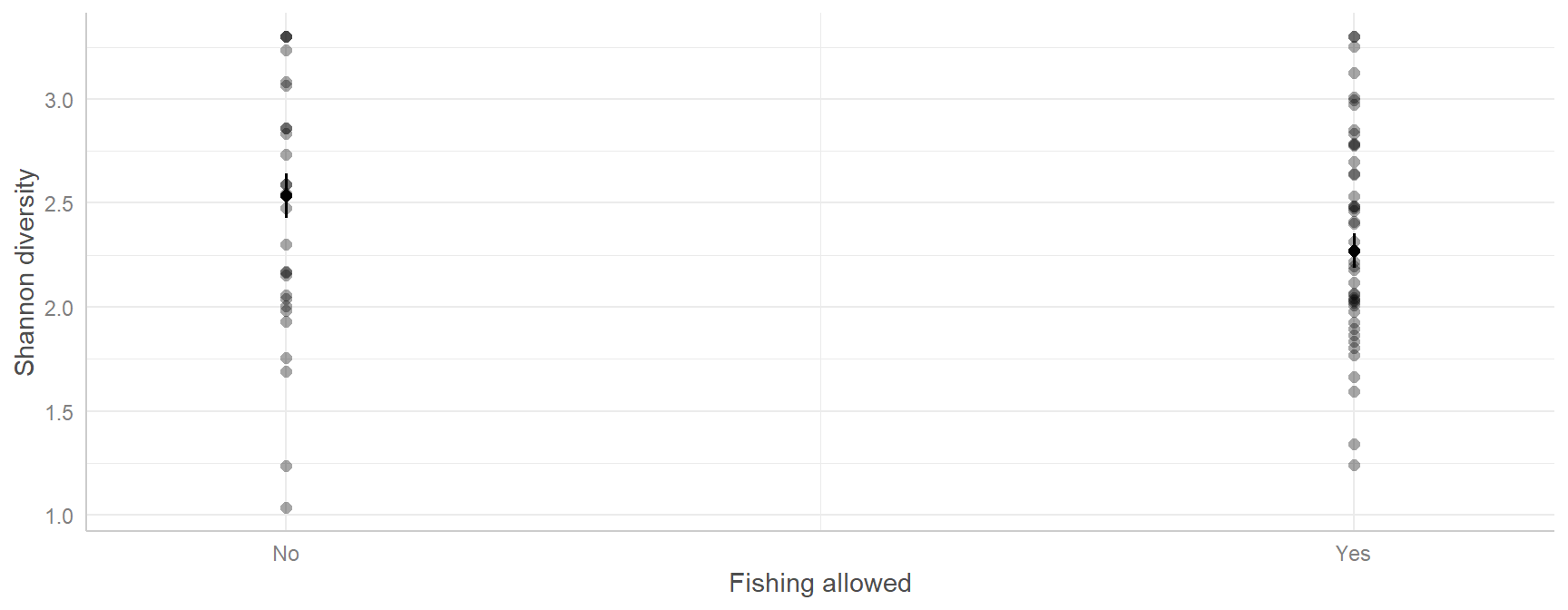
The best way to understand a multiple regression is to plot its predictions. ggeffects::predict_response() predicts diversity across the range of one predictor while holding the other predictors at their average (or reference level).

Code
# Predicted diversity across the observed range of each predictor
pred_chl  <- ggeffects::predict_response(reef_lm, terms = "chlorophyll")
pred_sst  <- ggeffects::predict_response(reef_lm, terms = "sst")
pred_fish <- ggeffects::predict_response(reef_lm, terms = "fishing_allowed")

pred_chl   # print the predictions: note the "Adjusted for" lines at the bottom
# Predicted values of shannon

chlorophyll | Predicted |     95% CI
------------------------------------
       0.00 |      3.63 | 3.43, 3.83
       0.20 |      2.89 | 2.77, 3.01
       0.40 |      2.15 | 2.03, 2.27
       0.60 |      1.41 | 1.22, 1.60

Adjusted for:
*             sst = 28.02
*              pH =  8.10
* fishing_allowed =    No
Code
# plot() draws each prediction with its 95% CI; show_data = TRUE adds the raw data
plot(pred_chl, show_data = TRUE) + ggplot2::labs(title = NULL, x = "Chlorophyll-a (mg/m³)", y = "Shannon diversity")

Code
plot(pred_sst, show_data = TRUE) + ggplot2::labs(title = NULL, x = "Sea surface temperature (°C)", y = "Shannon diversity")

Code
plot(pred_fish, show_data = TRUE) + ggplot2::labs(title = NULL, x = "Fishing allowed", y = "Shannon diversity")

5. Interpret

Each slope is the change in Shannon diversity for a one-unit increase in that predictor, holding all the other predictors constant:

Predictor Estimate 95% CI p Meaning
Chlorophyll -3.7 -4.24 to -3.16 < 0.001 Diversity drops by 0.37 for every 0.1 mg/m3 increase in chlorophyll
SST -0.26 -0.37 to -0.14 < 0.001 Diversity drops by 0.26 per 1 °C warmer
Fishing allowed (Yes vs No) -0.26 -0.4 to -0.13 < 0.001 Fished reefs are 0.26 lower in diversity
pH 5.93 -6.27 to 18.12 0.335 No clear effect: the CI is very wide and includes 0

A non-significant result for pH does not prove pH has no effect. pH varied very little among these sites (8.08–8.11), so the data contain little information about it.

Results sentence:

Coral diversity was lower at reefs with higher chlorophyll-a concentrations (β = -3.7, 95% CI -4.24 to -3.16, p < 0.001), higher sea surface temperatures (β = -0.26 per °C, 95% CI -0.37 to -0.14, p < 0.001) and where commercial fishing was allowed (0.26 lower, 95% CI 0.13–0.4, p < 0.001), but showed no clear relationship with pH (p = 0.34). Together these predictors explained 77% of the variation in diversity (F4,67 = 56.1, p < 0.001; Fig. 2). Distance from land was excluded because it was strongly correlated with chlorophyll (r = −0.97).

Assessment

Task to complete before the end of the workshop.

week07_assessment.R island.csv foraging_shrub.csv

Question 1. Island size and herbivore species richness (simple regression). Larger islands usually support more species (the species–area relationship). island.csv contains island area and herbivore species richness for 32 islands, in a similar way to Ross et al. (2019). Island area (island_area_log) is on the natural log scale, and species richness is given on both the raw (species_richness) and log (species_richness_log) scales.

  1. Plot raw species richness against log island area, then log species richness against log island area. Which looks more linear?
  2. Fit a linear model using the log-log version and check its assumptions.
  3. Report the slope and its 95% CI, the R2 and the p-value, and write a results sentence.
  4. Plot the data with the fitted line and its 95% CI.

Question 2. What determines fairy-wren foraging height? (multiple regression). foraging_shrub.csv records the foraging height (m) of superb fairy-wrens, the mean size of the surrounding shrubs (mean_shrub_size, a PCA score where larger values mean bigger shrubs), the bird’s sex (sex_mf) and the foraging substrate (substrate: air, bark, foliage or ground).

  1. Visualise the relationship between foraging height and each predictor.
  2. Fit a multiple regression with shrub size, sex and substrate as predictors (no interactions). Check the assumptions, including collinearity.
  3. Interpret the coefficient for mean_shrub_size and for sex_mfMale in words.
  4. Use ggeffects::predict_response() to plot predicted foraging height against shrub size.
  5. Extra (not marked): add an interaction between sex and substrate. Does it improve the model? What does it mean biologically?

Submit one R script (.R) before the end of the class. Write your answers to written questions as # comments next to the code that produced them.

Score What it looks like
0 No submission or no attempt.
0.25 Submitted, but a very poor attempt (e.g. incomplete, or lots of gaps).
0.5 Most questions answered, or all answered but most annotations missing.
0.75 All questions answered, but some annotations missing or some answers incorrect.
1 Everything completed, with annotations on all code so the marker can follow it.

Tip: an annotation is a short # comment that says what the line does and why. For example: # remove the one plant with a stem dry mass of 7.4 g (data entry error).

Additional resources

  • Coding Club: From distributions to linear models and Intro to model design.
  • Everything is a linear model.
  • Zuur et al. (2010) A protocol for data exploration to avoid common statistical problems: a short, practical checklist (outliers, collinearity, independence) to work through before any regression.
  • Zuur and Ieno (2016) A protocol for conducting and presenting results of regression-type analyses: how to report a regression clearly.
  • Dormann et al. (2013): a review of collinearity and the methods to deal with it.
  • Biostatistics with R (A. Terui): clear, ecology-focused notes on regression and GLMs.
  • Quinn & Keough (2002), chapters 5 (correlation and regression) and 6 (multiple regression).