2  Tidy Data

Week 2: Transforming and reshaping data, and writing tidy code

Raw data are rarely in exactly the form you need. Usually you need to keep some rows, drop some columns, calculate new variables, summarise by group or change the layout of the table. In this workshop you will learn the dplyr and tidyr functions that handle almost all of these jobs, and how to write code that other people (including future you) can read. Workshop materials are available in the GitHub repository ECS200.

TipLearning outcomes

By the end of this workshop you should be able to:

  1. Use filter(), arrange(), select(), mutate() and summarise() with group_by().
  2. Reshape data between wide and long format with pivot_longer() and pivot_wider().
  3. Chain several steps together with the pipe %>%.
  4. Write clean, consistent and well-annotated code.

Background

Five key dplyr functions (verbs) solve most data manipulation problems:

Verb What it does Example
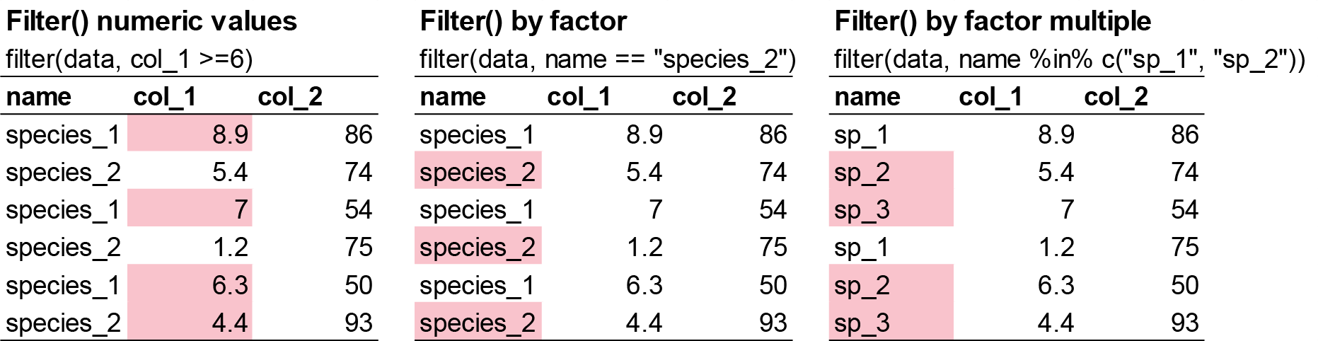
dplyr::filter() Keeps rows that meet a condition Keep seedlings from 2004
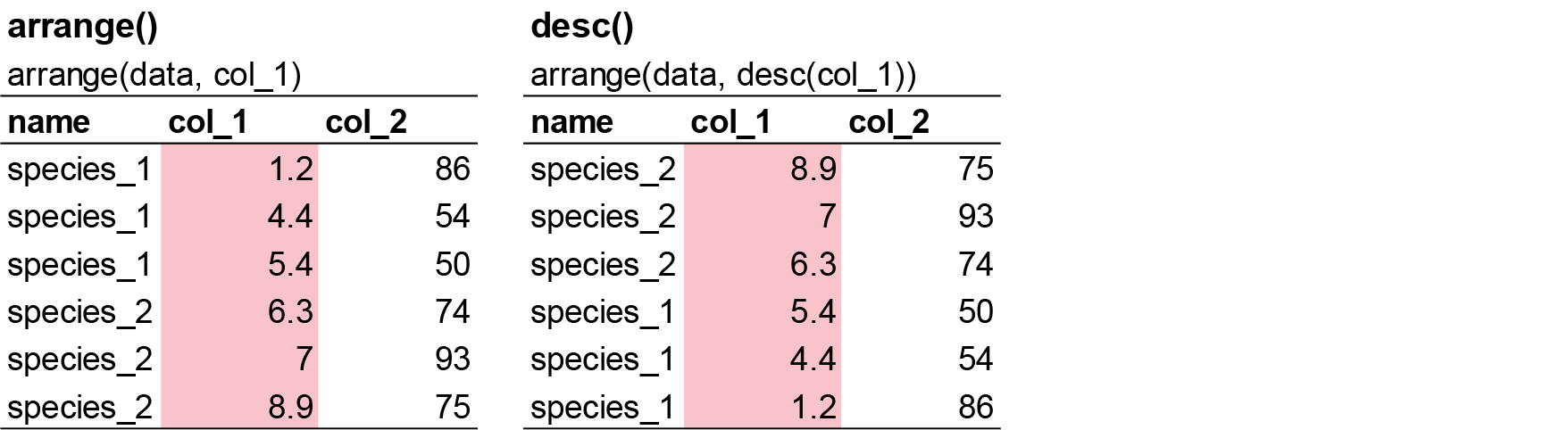
dplyr::arrange() Reorders rows Sort from the tallest to the shortest seedling
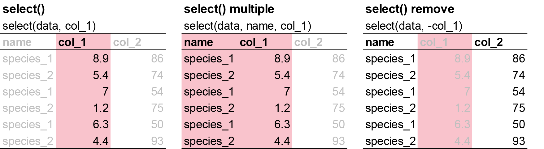
dplyr::select() Keeps (or drops) columns by name Keep only watershed and stem_length
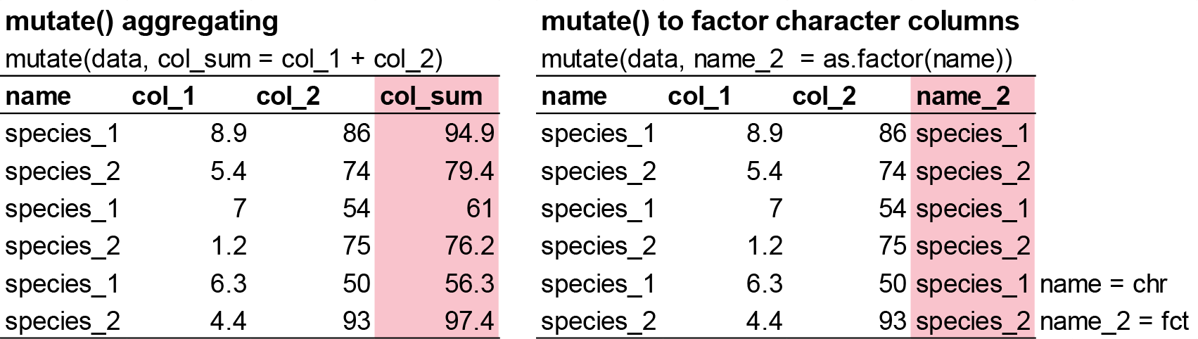
dplyr::mutate() Creates new columns from existing ones Total mass = leaf mass + stem mass
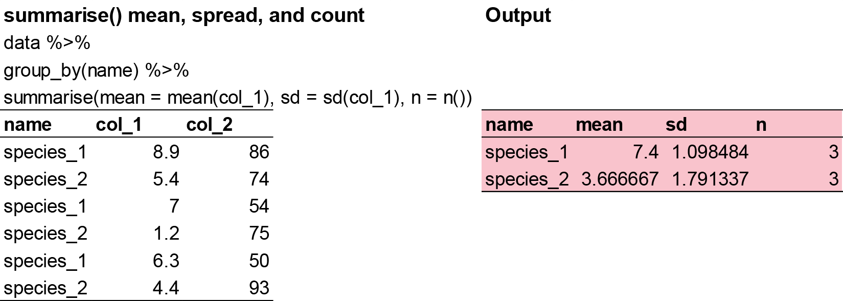
dplyr::summarise() Collapses many rows into a summary Mean stem length

All of them can be combined with dplyr::group_by(), which makes the next function work group by group (e.g. one mean per watershed instead of one overall mean).

All the verbs work the same way:

  • The first argument is a data frame (usually supplied by the pipe %>%).
  • The next arguments describe what to do, using column names without quotes.
  • The result is a new data frame.

Study context

We continue with the sugar maple data from Week 1. The dataset comes from the Hubbard Brook Experimental Forest in New Hampshire, USA.

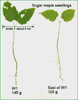
The growth of sugar maples (Acer saccharum) can be stunted by soil acidification from acid rain, which washes calcium (an important nutrient) out of the soil. To test whether adding calcium helps, researchers at the Hubbard Brook Long Term Ecological Research (LTER) site recorded “general sugar maple germinant health by height, leaf area, biomass, and chlorophyll content” (Juice et al., 2006) for seedlings in an untreated watershed (Reference) and a watershed treated with calcium in 1999 (W1) (Peters et al., 2004).

Sugar maple seedlings in the laboratory. Photo credit: Tom Siccama.

Part 1: Data manipulation

Start a new script and import the clean data you saved at the end of Week 1. If you did not finish Week 1, the code below recreates it from the raw file.

Code
# Week 2 workshop - Tidying data
# Written by Nicholas Wu, 1234578, 04/03/2027

library(tidyverse)

# setwd("C:/Users/YOUR-NAME/Documents/ECS200")

# Option 1: import the clean data you saved in Week 1
# plant_task_data_clean <- readr::read_csv("data/plant_task_data_clean.csv")

# Option 2: recreate the clean data from the raw file
plant_task_data_clean <- readr::read_csv("data/plant_calcium_task.csv") %>%
  dplyr::mutate(watershed = dplyr::if_else(watershed == "W2", "W1", watershed), # fix the mislabelled watershed
                watershed = factor(watershed),
                transect  = factor(transect)) %>%
  dplyr::filter(stem_dry_mass < 1)                                              # remove the data entry error

Exercise (15 min)

🧪 Use the functions above on fake_data

Code
fake_data <- data.frame(
  site = c("A", "B", "C", "A", "B", "A", "B", "C", "A", "B", "A", "B", "A", "B", "C", "C",
           "B", "A", "b", "C", "B", "C", "C", "A", "A", "A", "A", "B", "C", "C", "C"),
  species_1 = c(7, 25, 30, 50, 38, 13, 5, 31, 34, 22, 41, 25, 22, 37, 39, 13,
                45, 10, 40, 7, 28, 36, 19, 2, 12, 5, 16, 38, 27, 44, 44),
  species_2 = c(9, 8, 1, 7, 9, 9, 4, 8, 1, 7, 1, 6, 4, 4, 7, 2,
                8, 7, 2, 9, 9, 2, 6, 8, 6, 6, 17, 1, 8, 4, 4),
  species_3 = c(190, 160, 70, 430, 310, 99, 530, 420, 371, 357, 198, 171, 463, 124, 254, 484,
                435, 409, 122, 305, 410, 162, 473, 200, 401, 273, 421, 419, 293, 487, 487),
  species_4 = c(2, 0, 4, 8, 6, 3, 7, 4, 2, NA, 35, 10, 6, 4, 8, 1,
                1, 0, NA, 4, 6, 8, 10, 6, 2, 5, 10, 7, NA, NA, NA)
)
  • Run the usual quality check (the mistakes are slightly different from Week 1).
  • Create a new column called total_sp that adds up all four species.
  • Keep only the site and total_sp columns.
  • Calculate the mean, minimum, maximum and number of samples of total_sp for each site.

Questions:

  1. What is the mean total abundance at site B?
  2. These are counts of individuals. Is the mean a sensible summary? (Hint: think about decimals.)
  3. Which site has the highest average abundance?
  4. Which site has the most samples?
Show answer
Code
# Quality check: "b" should be "B", species_4 has NAs and one extreme value (35)
fake_data_clean <- fake_data %>%
  dplyr::mutate(site = dplyr::if_else(site == "b", "B", site), # fix the label
                site = factor(site)) %>%
  dplyr::filter(species_4 < 30) %>%                             # removes the extreme value AND the NA rows
  dplyr::mutate(total_sp = species_1 + species_2 + species_3 + species_4) %>%
  dplyr::select(site, total_sp)

fake_data_clean %>%
  dplyr::group_by(site) %>%
  dplyr::summarise(mean = mean(total_sp),
                   min  = min(total_sp),
                   max  = max(total_sp),
                   n    = dplyr::n())
# A tibble: 3 × 5
  site   mean   min   max     n
  <fct> <dbl> <dbl> <dbl> <int>
1 A      355.   124   495    10
2 B      361.   169   546     8
3 C      345.   105   508     7
Code
# 1. 361.25
# 2. A mean of a count can be a decimal (e.g. 361.25 individuals). The median
#    is often a better summary for counts, especially if they are skewed.
# 3. Site B
# 4. Site A

Note that filter(species_4 < 30) also removes rows where species_4 is NA, because R cannot tell whether NA < 30. That is fine here, but be aware of it.

Part 2: Reshaping data

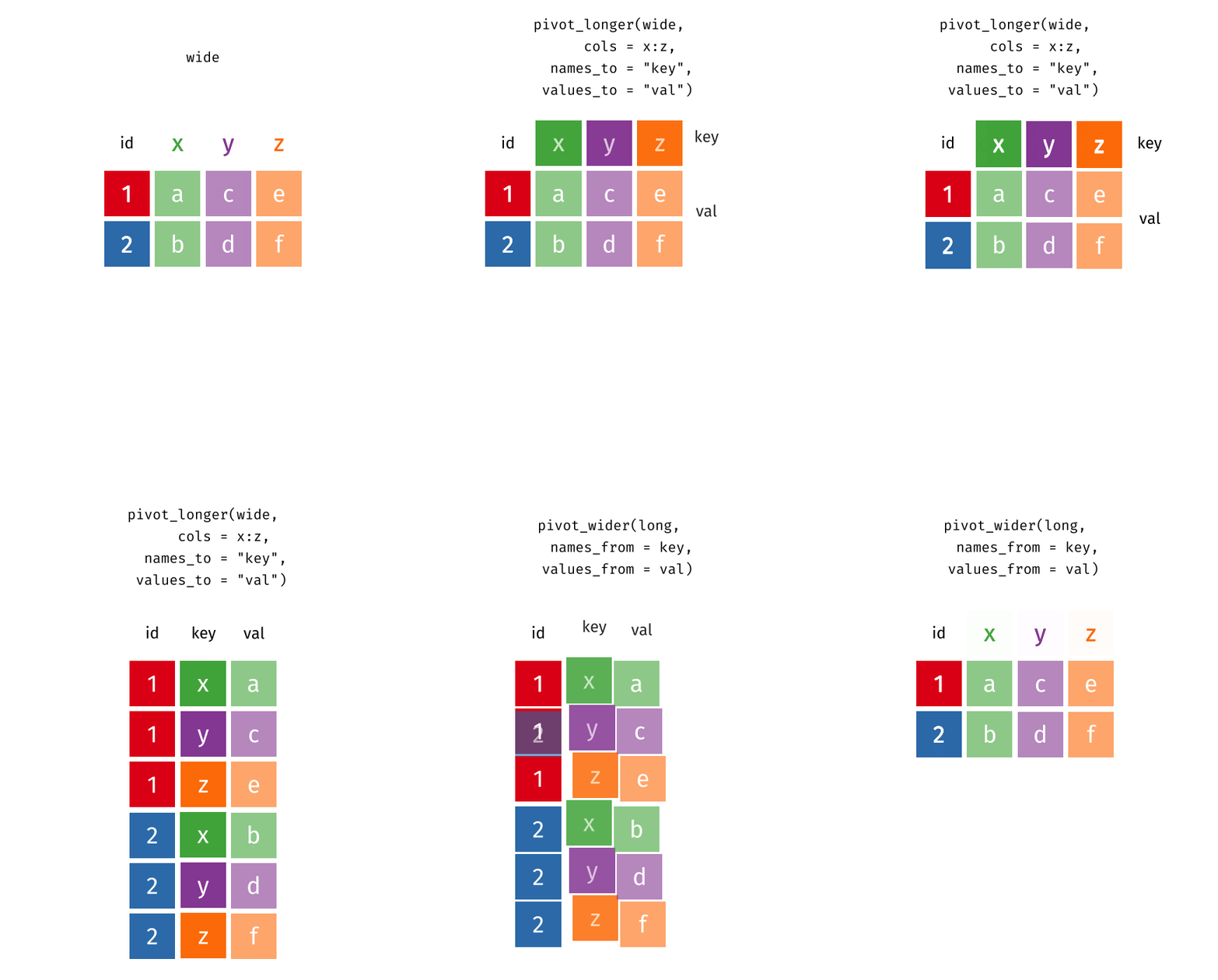
Recall from Week 1 that tidy data have one row per observation. Field data sheets are often in wide format (e.g. one column per species or per month), while most tidyverse functions, and every statistical model, need long format.

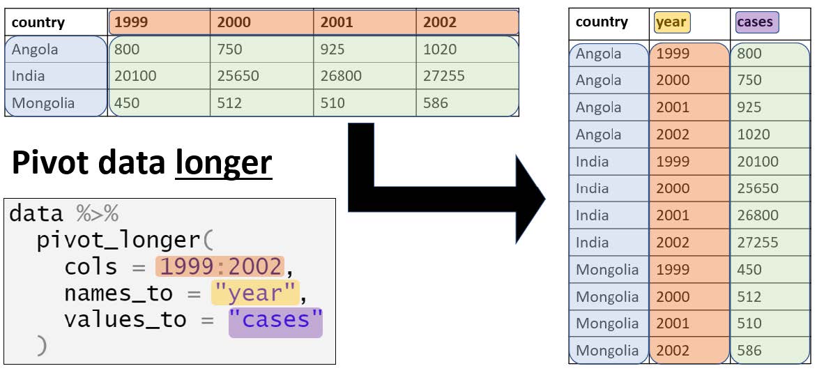
tidyr::pivot_longer() turns wide data into long data. The column names become values in a new column (names_to) and the cell values go into another new column (values_to).

Code
# A wide table: one column per month
wide_data <- data.frame(site = c("A", "B"),
                        jan  = c(10, 20),
                        feb  = c(15, 25))
wide_data
  site jan feb
1    A  10  15
2    B  20  25
Code
# Long format: one row per site and month
long_data <- wide_data %>%
  tidyr::pivot_longer(cols      = jan:feb,   # the columns to stack
                      names_to  = "month",   # new column for the old column names
                      values_to = "count")   # new column for the values
long_data
# A tibble: 4 × 3
  site  month count
  <chr> <chr> <dbl>
1 A     jan      10
2 A     feb      15
3 B     jan      20
4 B     feb      25

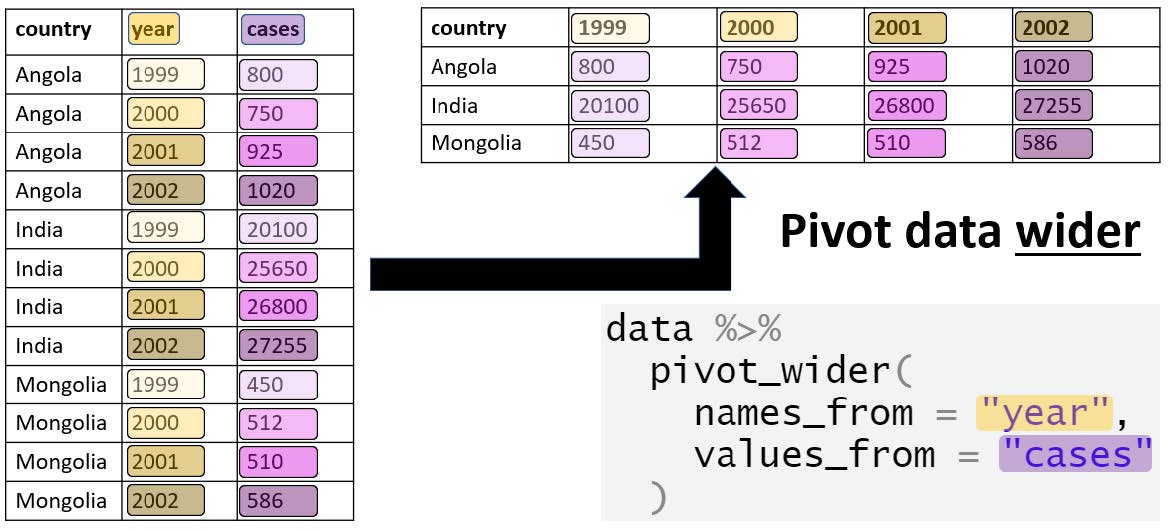
tidyr::pivot_wider() does the opposite. It is useful for making summary tables that are easy to read in a report.

Code
long_data %>%
  tidyr::pivot_wider(names_from  = month,  # the column whose values become new column names
                     values_from = count)  # the column whose values fill the cells
# A tibble: 2 × 3
  site    jan   feb
  <chr> <dbl> <dbl>
1 A        10    15
2 B        20    25

Exercise (5 min)

🧪 Convert fake_data to long format, with one row per sample and species and columns called species and abundance. How many rows does the long version have, and why?

Show answer
Code
fake_long <- fake_data %>%
  tidyr::pivot_longer(cols      = species_1:species_4,
                      names_to  = "species",
                      values_to = "abundance")

nrow(fake_long) # 31 samples x 4 species = 124 rows
[1] 124

Part 3: Tidy code

Good coding style is like correct punctuation: you can manage without it, butitsuremakesthingseasiertoread. The most important rule is to be consistent. We follow the tidyverse style guide.

Exercise (15 min)

🧪 Clean someone else’s code

Your colleague has left for a new job and you have taken over their project. They ran a quick analysis but did not do a quality check, the code does not run, and the comments are unclear. Fix the code so it runs, add a quality check, and improve the comments.

Code
# Exercise 2
# Cleaning code and tidying dataset
# John Smith, 25-03/2025

## Set up ## ----------------------------------------------------------------
library(tiderVerse)

# Set my directory
setwd("YOUR DIRECTORY")

## Loading and cleaning data ## ---------------------------------------------

# Load raw data
plant data <- read_csv("data/plant_calcium.csv")
str(plant data)

## Analysis ## -------------------------------------------------------------

# Fit model: height explained by elevation
model <- lm(stem_dry_mass ~ stem_length, data = plant_data)

# Check model summary
summary(model)

## Visualisation ## --------------------------------------------------------

# Creating scatterplot figure
plant_data %>%
  ggplot() +
  geom_point(aes(x = stem_length, y = Stem_dry_mass)) +
  labs(
    x = "Stem Length (mm)",
    y = "Stem Dry Mass (g)",
    title = "Stem Dry Mass vs. Stem Length in Sugar Maple Seedlings",
    subtitle = "Hubbard Brook LTER"
  ) +
  theme_minimal()
Show answer
Code
# Relationship between stem length and stem dry mass in sugar maple seedlings
# Cleaned version of John Smith's script (original 25/03/2025)
# YOUR NAME, DATE

## Set up ## ------------------------------------------------------------------
library(tidyverse)          # fixed the package name (was "tiderVerse")

# setwd("YOUR-WORKSHOP-FOLDER")

## Load and clean data ## -----------------------------------------------------

# Object names cannot contain spaces (was "plant data")
plant_data <- readr::read_csv("data/plant_calcium.csv")
dplyr::glimpse(plant_data)

# Categorical variables to factors
plant_data <- plant_data %>%
  dplyr::mutate(watershed = factor(watershed),
                elevation = factor(elevation))

# Quality check: missing values, duplicates and outliers
colSums(is.na(plant_data))      # NAs in elevation and the leaf area columns, but not in the columns we analyse
sum(duplicated(plant_data))     # no duplicated rows

ggplot2::ggplot(plant_data, ggplot2::aes(x = stem_dry_mass)) +
  ggplot2::geom_histogram(bins = 30)  # no impossible values

## Analysis ## ----------------------------------------------------------------

# Linear model: stem dry mass explained by stem length (the old comment was wrong)
stem_mass_lm <- lm(stem_dry_mass ~ stem_length, data = plant_data)
summary(stem_mass_lm)

## Figures ## -----------------------------------------------------------------

# Scatterplot (column names are case sensitive: stem_dry_mass, not Stem_dry_mass)
plant_data %>%
  ggplot2::ggplot() +
  ggplot2::geom_point(ggplot2::aes(x = stem_length, y = stem_dry_mass)) +
  ggplot2::labs(x        = "Stem length (mm)",
                y        = "Stem dry mass (g)",
                title    = "Stem dry mass vs. stem length in sugar maple seedlings",
                subtitle = "Hubbard Brook LTER") +
  ggplot2::theme_minimal()

Assessment

Task to complete before the end of the workshop.

week02_assessment.R

Use your plant_task_data_clean.csv from Week 1 (or recreate it with the code at the top of this page).

  1. Keep only these columns: year, watershed, elevation, stem_length, leaf_dry_mass and stem_dry_mass.
  2. Create a new column, total_mass_mg, with the total dry mass (leaf + stem) of each seedling in milligrams.
  3. Create a summary table with the mean, standard deviation and sample size of total_mass_mg for each combination of watershed and year.
  4. Use tidyr::pivot_wider() to turn the means from your summary table into a table with one row per watershed and one column per year.
  5. Interpretation: did seedlings in the calcium-treated watershed (W1) have a higher mean total mass than seedlings in the Reference watershed in both years? By roughly how much? (Answer as comments.)
  6. Save this script. In Week 3 you will continue from it under a new header: “Week 3 workshop - Descriptive statistics”.

Submit one R script (.R) before the end of the class. Write your answers to written questions as # comments next to the code that produced them.

Score What it looks like
0 No submission or no attempt.
0.25 Submitted, but a very poor attempt (e.g. incomplete, or lots of gaps).
0.5 Most questions answered, or all answered but most annotations missing.
0.75 All questions answered, but some annotations missing or some answers incorrect.
1 Everything completed, with annotations on all code so the marker can follow it.

Tip: an annotation is a short # comment that says what the line does and why. For example: # remove the one plant with a stem dry mass of 7.4 g (data entry error).

For the adventurous

  1. Write one pipe that keeps W1 seedlings from 2004, calculates total_mass_mg, keeps only total_mass_mg and stem_length, keeps seedlings taller than 100 mm, and sorts from heaviest to lightest.
  2. In one pipe, group by watershed and year and calculate the mean, the coefficient of variation (SD / mean × 100) and the sample size of total_mass_mg.

Extra: operators and joins

Common operators used inside dplyr::filter():

Operator Meaning
== Equal to
!= Not equal to
<, <= Less than, less than or equal to
>, >= Greater than, greater than or equal to
%in% Matches any value in a list, e.g. site %in% c("A", "B")
& AND: both conditions must be true
| OR: at least one condition must be true
! NOT, e.g. !is.na(x) keeps non-missing values

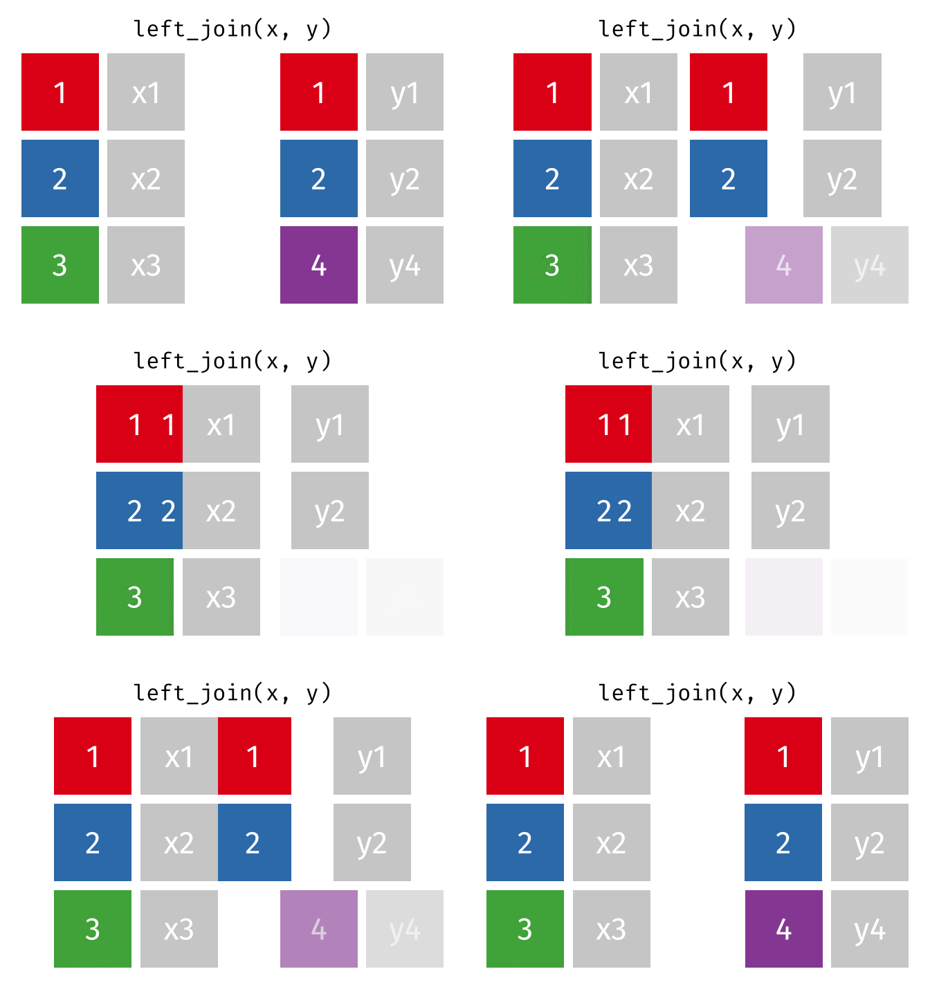
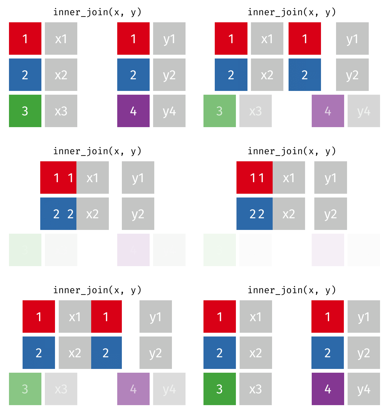
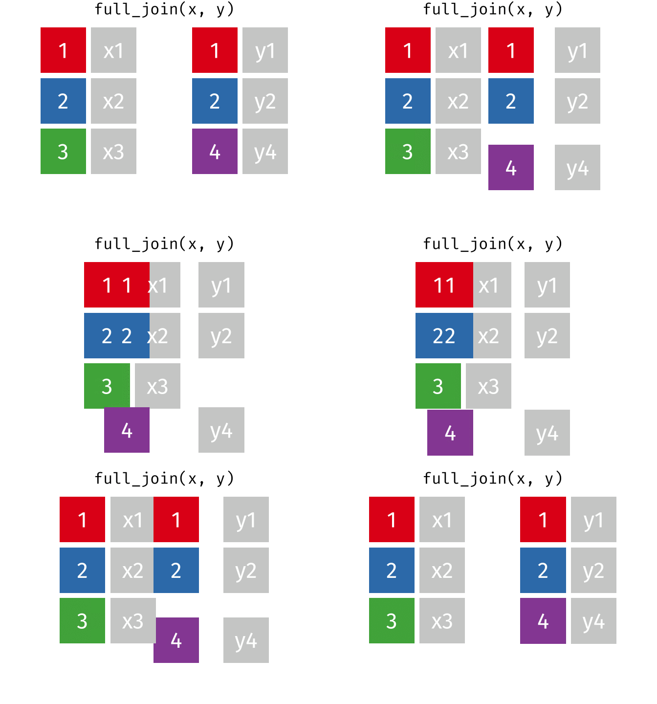
Joins combine two data frames that share a “key” column, e.g. a table of plots and a separate table of plot soil properties.

Additional resources