Research Design

Good analysis cannot rescue a poor design. Most of the problems you will meet in Weeks 5–13 (non-independent data, confounded treatments, too few replicates, false zeros) are much easier to prevent when you plan a study than to fix after the data are collected. This appendix adds to the lecture notes on research design, with a focus on designing studies that are easy to analyse.

From question to analysis

Plan your analysis before you collect data. Four principles for sound statistical ecology (Popovic et al., 2024):

  1. Define a focused research question, then plan the sampling and the analysis to answer it.
  2. Use a model that accounts for the distribution and dependence of your data (counts → Week 8, yes/no → Week 11, grouped or repeated measurements → Week 12).
  3. Emphasise effect sizes (how big is the effect, with a confidence interval) rather than only whether p < 0.05.
  4. Report your methods and results in enough detail that someone else could repeat the study and use your results (Davis and Kay, 2023; Gerstner et al., 2017).

A useful exercise: before collecting any data, sketch the figure you expect to make and write the R model formula you plan to fit, e.g. lm(sprint_speed ~ temperature * population). If you cannot write the formula, the design is not finished yet.

Who or what are you making conclusions about?

The scope of inference is the “population” your conclusions apply to. Define it in three dimensions before you sample:

  • Spatial: one wetland, all wetlands on the Swan Coastal Plain, or all of south-west WA?
  • Temporal: one breeding season, or long-term conditions? A question about a 10-year cycle needs more than one year of data.
  • Ecological: one species, one life stage, or a whole community?

Your sample can only represent the population you actually sampled from. Larger and more variable populations need more samples.

Replicate at the right scale

The most important design decision is the experimental (or sampling) unit: the smallest unit to which a treatment is independently applied, or that is independently sampled. Replication must happen at the same scale as the treatment (Hurlbert, 1984; Marshall, 2024).

Design Treatment applied to True replicate Pseudoreplicates (subsamples)
Nutrients added to individual pots Pot Pot Several leaves per plant
Water heated in a tank holding 5 snails Tank Tank The 5 snails
Fire applied to whole plots Plot Plot Quadrats within each plot
Comparing burnt and unburnt sites Site Site Traps within each site
Comparing high and low pH populations Population Population Individuals within a population

Subsamples are useful (they give a better estimate for each unit), but they are not independent replicates. Either average them for each experimental unit, or include the unit as a random effect (Week 12).

NoteLink to your project

On The Islands, each plot is the experimental unit for a nutrient treatment. Ten plants measured in one plot are not ten replicates. And if you compare islands, you have only one field station per island, so island and climate are completely confounded: any difference could be caused by climate, soil, or anything else that differs between the islands. Say so clearly in your report.

Randomise, intersperse and block

  • Randomise which units get which treatment, so unmeasured differences (soil, shade, observer) are spread evenly among treatments. Use R to do it:
Code
# Randomly assign 3 nutrient treatments to 36 plots (12 plots each)
set.seed(2027)  # makes the randomisation repeatable; change the number for your own design
plot_design <- data.frame(
  plot      = 1:36,
  treatment = sample(rep(c("control", "low N", "high N"), each = 12)) # shuffle the 36 labels
)
head(plot_design)
  plot treatment
1    1   control
2    2   control
3    3    high N
4    4     low N
5    5    high N
6    6     low N
  • Intersperse treatments in space and time. Putting all the controls in one row, or measuring all controls in the morning and all treatments in the afternoon, confounds the treatment with location or time.
  • Block when there is a known gradient (e.g. slope, distance from the coast). Group similar units into blocks and assign every treatment within each block. Block then becomes a random effect (Week 12) or a fixed factor in the analysis.

Controls and before–after designs

To measure the effect of an impact (mining, fire, restoration), you need to know what would have happened without it. Simple designs often give wrong answers: an analysis of hundreds of ecological datasets found that before–after or control–impact designs alone can be very inaccurate, and that before–after control–impact (BACI) and randomised designs were much more reliable (Christie et al., 2019; Christie et al., 2020). Where possible, collect data before the impact at both impact and control sites, and use several control sites. Experiments built into management actions are one of the best ways to get this evidence (Ockendon et al., 2021). The Controls app below shows why.

Design decisions determine the analysis

If your design has… …you will need Week
Two or more groups and a continuous response t-test or ANOVA 5
A numeric predictor (gradient) Linear regression 7
Several correlated predictors Choose predictors carefully, check VIF 7
Counts (individuals, species, seeds) Poisson or negative binomial GLM 8
Unequal effort among samples (trap nights, area) An offset in a GLM: record the effort! 8
Yes/no responses (present, survived, bleached) Logistic regression 11
Several measurements per individual, site or tank Mixed-effects model 12
Time until an event, with some individuals not reaching it Survival analysis 13

How many samples do I need?

Statistical power is the probability that a study will detect an effect (p < 0.05) if the effect is real. Studies with low power often miss real effects, and when they do find something, they tend to overestimate it. A common target is 80% power.

Power depends on four things:

  1. Effect size: the smallest difference that would matter biologically. Decide this from the literature or from what would matter for management, not from what you hope to find.
  2. Variability (SD) of the response. Estimate it from a pilot study, previous studies or similar data.
  3. Sample size (n).
  4. Significance level (α, usually 0.05).

Choose three of them, and you can calculate the fourth. Use the app to see how they trade off.

App: statistical power and sample size (two-group comparison)

Power analysis in R

Base R has functions for the simplest designs. Leave out the one quantity you want R to calculate.

Two groups (t-test): the lizard experiment in Week 5. Suppose a pilot study gave an SD in sprint speed of 0.25 m/s, and a difference of 0.3 m/s between temperatures would be biologically important. How many lizards per temperature?

Code
power.t.test(delta = 0.3, sd = 0.25, power = 0.8, sig.level = 0.05)

     Two-sample t test power calculation 

              n = 11.94228
          delta = 0.3
             sd = 0.25
      sig.level = 0.05
          power = 0.8
    alternative = two.sided

NOTE: n is number in *each* group

Round up: 12 lizards per group. And what power would you have with only 10 per group?

Code
power.t.test(n = 10, delta = 0.3, sd = 0.25, sig.level = 0.05)

     Two-sample t test power calculation 

              n = 10
          delta = 0.3
             sd = 0.25
      sig.level = 0.05
          power = 0.7184022
    alternative = two.sided

NOTE: n is number in *each* group

Three or more groups (one-way ANOVA): give the expected group means and the within-group variance (SD2):

Code
# Expected mean sprint speed at 20, 28 and 36 C, and a within-group SD of 0.25
expected_means <- c(1.2, 1.8, 1.6)

power.anova.test(groups      = 3,
                 between.var = var(expected_means),  # variance among the expected means
                 within.var  = 0.25^2,                # SD squared
                 power       = 0.8)

     Balanced one-way analysis of variance power calculation 

         groups = 3
              n = 4.395181
    between.var = 0.09333333
     within.var = 0.0625
      sig.level = 0.05
          power = 0.8

NOTE: n is number in each group

For GLMs, mixed models and other complex designs there is no simple formula. Instead, simulate the study many times with your planned sample size and effect, analyse each simulated dataset, and count how often the effect is significant. This is optional, but it is a very powerful way to plan a study.

Example: will 20 plots per treatment detect a 30% increase in fruit number (from a mean of 5 to 6.5 fruits per plant) with a Poisson GLM?

Code
set.seed(1)
n_per_group <- 20       # plots per treatment
n_sims      <- 500      # number of simulated studies
p_values    <- numeric(n_sims)  # empty vector to store each study's p-value

for (i in 1:n_sims) {
  # 1. Simulate one study
  sim_data <- data.frame(treatment = rep(c("control", "fertilised"), each = n_per_group))
  sim_data$fruits <- rpois(n = 2 * n_per_group,
                           lambda = ifelse(sim_data$treatment == "control", 5, 6.5))
  # 2. Analyse it
  sim_model <- glm(fruits ~ treatment, family = poisson, data = sim_data)
  # 3. Store the p-value for the treatment effect
  p_values[i] <- summary(sim_model)$coefficients["treatmentfertilised", "Pr(>|z|)"]
}

# Power = proportion of simulated studies with p < 0.05
mean(p_values < 0.05)
[1] 0.522

Only about half of the simulated studies detect the effect, so 20 plots per treatment is not enough. Increase n_per_group and run it again to find the sample size that gives 80% power. Real counts are usually overdispersed (Week 8), so you would need even more.

How much survey effort?

For surveys, “sample size” also means effort: how many visits, traps or quadrats.

Detecting a species that is present. If a species is detected with probability p on a single visit when it is present, the chance of missing it on k visits is (1 − p)k. To be 95% sure of detecting it:

\[ k = \frac{\log(1 - 0.95)}{\log(1 - p)} \]

Code
# Number of visits needed to be 95% sure of detecting a species that is present,
# for single-visit detection probabilities of 0.1 to 0.9
detection <- data.frame(p_detect = seq(0.1, 0.9, by = 0.1)) %>%
  dplyr::mutate(visits_needed = ceiling(log(1 - 0.95) / log(1 - p_detect)))

detection
  p_detect visits_needed
1      0.1            29
2      0.2            14
3      0.3             9
4      0.4             6
5      0.5             5
6      0.6             4
7      0.7             3
8      0.8             2
9      0.9             2

A cryptic frog detected on 30% of visits needs 9 visits per site before “not detected” reasonably means “absent”. With fewer visits, many of your zeros will be false zeros (see below). Occupancy designs that repeat visits only where a species has not yet been detected can save a lot of effort for rare species (Specht et al., 2017).

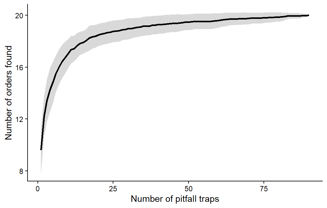
Finding most of the species in a community. A species accumulation curve shows how many species you find as you add samples. When the curve flattens, extra samples add few new species.

Code
# Invertebrate pitfall data from Week 4: one row per trap, one column per order
invert_matrix <- readr::read_csv("data/invert_exp_survey.csv") %>%
  dplyr::select(Blattodea:Annelida)

# Expected number of orders found for 1, 2, 3... traps (random order of traps)
invert_accum <- vegan::specaccum(invert_matrix, method = "random")

accum_data <- data.frame(traps    = invert_accum$sites,
                         richness = invert_accum$richness,
                         sd       = invert_accum$sd)

ggplot2::ggplot(accum_data, ggplot2::aes(x = traps, y = richness)) +
  ggplot2::geom_ribbon(ggplot2::aes(ymin = richness - sd, ymax = richness + sd), fill = "grey85") +
  ggplot2::geom_line(linewidth = 1) +
  ggplot2::labs(x = "Number of pitfall traps", y = "Number of orders found") +
  ggplot2::theme_classic()

Here, about 20 traps find most of the orders, and the remaining traps add only rare ones.

NoteLink to your project

Each Island field station has 36 plots. More treatment levels means fewer replicates per treatment: 2 treatments give 18 plots each, 3 give 12, 4 give 9 and 6 give 6. Use power.t.test() or power.anova.test(), with an SD from the literature or a pilot run, to check whether your design has a reasonable chance of detecting the effect you care about before you plant anything.

Zeros and NAs in R

Ecological data are messy, but R doesn’t care: rubbish in, rubbish out. When designing surveys, it is essential to distinguish carefully between “0” and “NA” in your data sheet, because they mean completely different things.

  • Record a 0 only when a site was actually sampled with adequate effort and the species was not detected. Sampling happened, detection was possible, and the count was zero. A zero is data.
  • Record an NA when the site was not sampled, sampling failed, effort was inadequate, or the value is otherwise missing. An NA means “we do not know”.

Mixing them up causes real problems:

  • Coding a missing value as 0 claims a confirmed absence. This biases occupancy or abundance estimates downwards, adds extra zeros and can lead you to fit the wrong model (e.g. a zero-inflated model when the real problem is missing data). If your pH meter broke, the pH of those samples is unknown, not 0.
  • Coding a true zero as NA means R drops that observation from many analyses (e.g. tidyr::drop_na()), reducing your sample size and biasing results.

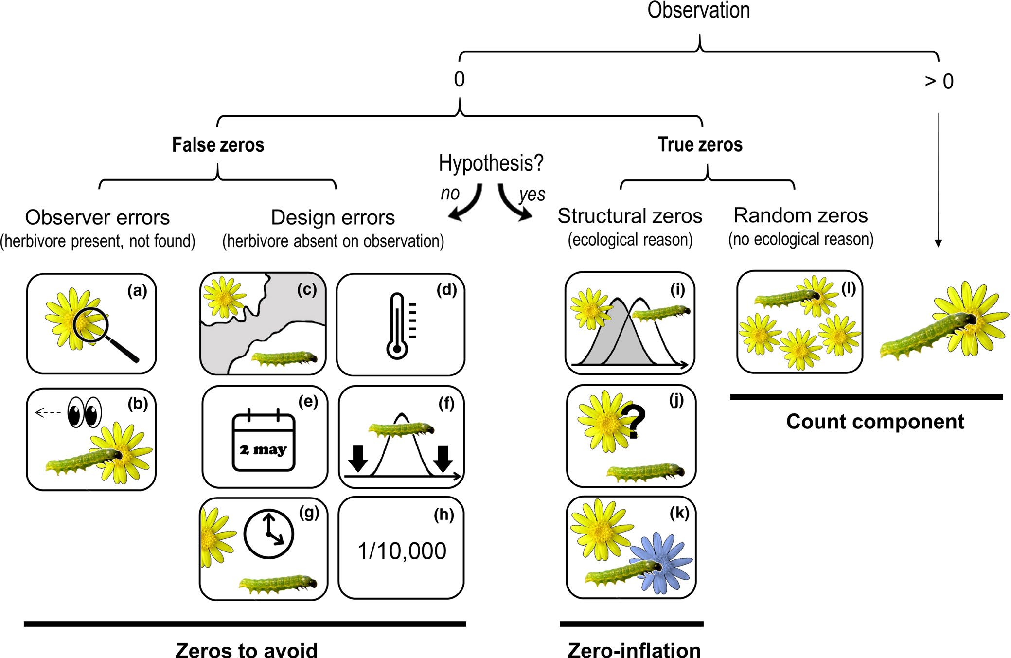
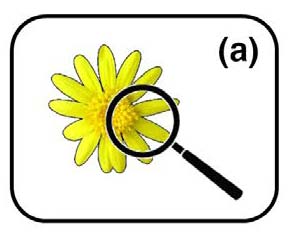
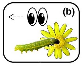
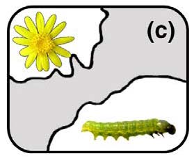
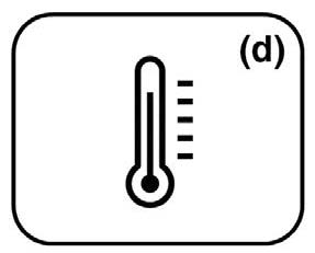
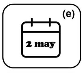
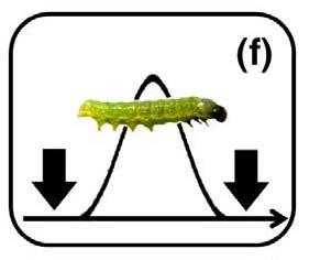
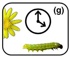
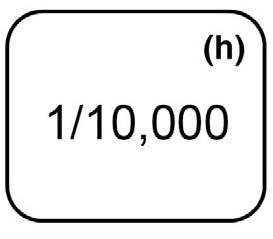
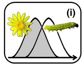
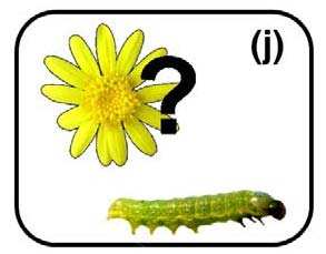
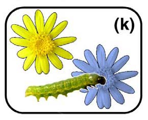
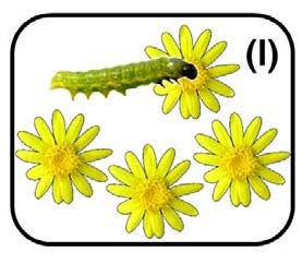
Zeros can arise in different ways (Blasco-Moreno et al., 2019). In the example below (herbivorous insect species on a plant species), zeros caused by an inexperienced observer (a–b) or by a poor design (c–h) are false zeros, which should be minimised through good design. Structural zeros, caused by the biology of the system (i–k), and random zeros from sampling variation (l) are true zeros.

Sources of zeros in count data. From Blasco-Moreno et al. (2019), Figure 1.

The scenarios that produce a zero, and how to minimise false zeros:

Scenario Type How to reduce it
The insects or their damage are too small for the observer to detect False Sample when insects are well developed
The observer misses the herbivore (e.g. mistakes it for a seed) or attributes damage to another cause False Train observers
The distributions of the herbivore and the plant do not overlap False Know the species’ distributions before sampling
The herbivore is absent from a location within its range (e.g. unsuitable microclimate) False Sample suitable habitats, or replicate surveys across areas
A single survey does not coincide with the herbivore’s life cycle False Know the life cycle, or survey repeatedly
A long-term survey samples too infrequently to catch the herbivore False Sample more often
Herbivores are absent at the time of sampling False Record plant damage instead of insects
Herbivores are so rare that the design cannot detect them False Sample more extensively, with more replicates
Plant and herbivore phenologies do not overlap True (structural) –
Herbivores do not recognise the plant as a host True (structural) –
Herbivores prefer another host species True (structural) –
The herbivore population is too small to use all the plants True (random) –

Common statistical mistakes

Most mistakes in published research are not failures of advanced mathematics. They are everyday errors of design and interpretation that are easy to make and easy to miss (Makin and Orban de Xivry, 2019). Each tab below has an app: move the sliders, press Resample and watch how the conclusion can change, often dramatically, from nothing more than chance, sample size or a decision made by the researcher. The apps were inspired by BIOL 3P96 Biostatistics.

Recording and reporting

  • Design your data sheet for analysis: one row per observation, one column per variable (Week 1), with a unique ID for every sampling unit and columns for the grouping structure (site, plot, individual, block) and effort (trap nights, area, minutes).
  • Keep a metadata file that explains every column, its units, and how NAs and zeros were recorded.
  • Write methods that someone else could repeat: the sampling unit, sample sizes, the model (response, predictors, distribution, random effects), how assumptions were checked, and the software and packages used (Davis and Kay, 2023; Rowe, 2023).
  • Report results that others can reuse: means, SDs and sample sizes for each group, effect sizes with confidence intervals and exact p-values, even for non-significant results. This lets your study be included in future meta-analyses (Gerstner et al., 2017).

Additional resources

  • Marshall (2024) Principles of experimental design for ecology and evolution: a short, clear guide to choosing the right scale of replication.
  • Popovic et al. (2024) Four principles for improved statistical ecology.
  • Steel et al. (2013) Applied statistics in ecology: common pitfalls and simple solutions, and Steel et al. (2019) on thinking statistically rather than just calculating.
  • Christie et al. (2019): why BACI and randomised designs give more accurate answers.
  • Ockendon et al. (2021): how to build experiments into conservation management.
  • Blasco-Moreno et al. (2019): understanding false, random and structural zeros.
  • Makin and Orban de Xivry (2019): ten common statistical mistakes to watch out for.
  • Quinn & Keough (2002), chapter 7 (design and power analysis).
  • Coding Club: Intro to model design.