The Islands
The Islands is a virtual environment originally designed for students to collect data to answer questions in epidemiology. It has since been updated to include field stations that allow for plant growth. The plants can represent any plant species: an agriculturally important plant, a plant of cultural significance to Indigenous people, a species of conservation concern or a pest species. You will decide on what plant it is and how it is related to your topic.
Note: the plants grow in real time, and typically take at least 14 days to fully grow, depending on the local climate.
Access The Islands from myMurdoch Learning under the ‘Group Project’ tab.
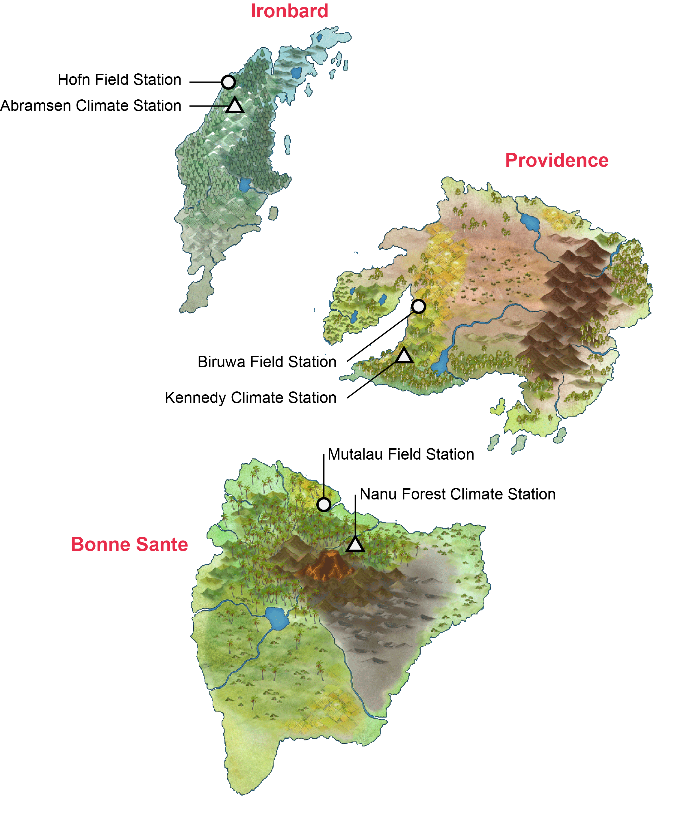
There are three islands in this world, each occupied by human settlers and each with a plant field station and a weather station (Fig. 1):
Ironbard: Ironbard is the most northern island and has a temperate climate (equivalent to Tasmania’s climate). The plant field station in Ironbard is called Hofn Field Station. The local weather station is called Abramsen Climate Station.
Providance: Providance is the eastern island and has a semi-arid climate (equivalent to Perth’s climate). The plant field station in Providance is called Biruwa Field Station. The local weather station is called Kennedy Climate Station.
Bonne Sante: Bonne Sante is the most southern island and has a subtropical climate (equivalent to Brisbane’s climate). The plant field station in Bonne Sante is called Mutalau Field Station. The local weather station is called Nanu Forest Climate Station.
Altogether, there are three field stations from three islands with differing climates. Each station has 36 plots.
Design your project
Design your experiment as if it were a real experiment. First, choose a plant species to tell your story.
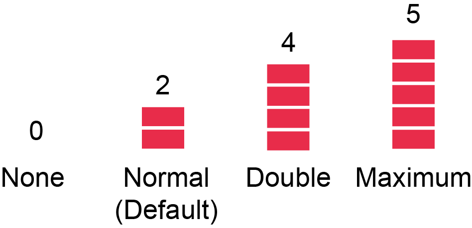
Next, you can manipulate nitrogen (N) and phosphorus (P) levels in the soil prior to growing the plants. The levels of N and P are represented by ‘blocks’. Two blocks is the default setting, which represents normal levels of N and P (Fig. 2). No blocks means no N or P, four blocks means twice the concentration of normal levels, and five blocks is the maximum allowed (represents 2.5 times normal levels). Give the blocks some values (e.g. milligram nitrogen per kilogram of soil; mg/kg). Use realistic values based on the literature and what is considered normal for the plant of interest.
Because there are three stations that span across different climates, you can compare the effects of temperature or rainfall on plant growth, fruit production, etc. All stations provide the date, maximum temperature in degrees Celsius and rainfall in millimetres (Table 1). You can relate these data to your dependent variables. You have the option to look at the interaction of N or P with temperature or rainfall (factorial design).
| Date | Max Temp (°C) | Rainfall (mm) |
|---|---|---|
| 01/064 | 18.8 | 1.0 |
| 02/064 | 23.7 | 0.8 |
| 03/064 | 25.3 | 0.8 |
| 04/064 | 29.3 | 0.0 |
| 05/064 | 29.7 | 14.1 |
With 36 plots per station, you can have 18 replicate plots per treatment if you have two treatments, 12 replicate plots per treatment if you have three treatments, 9 replicate plots per treatment if you have four treatments, and 6 replicate plots per treatment if you have six treatments. Balance the number of treatments against the number of replicates. The Research Design appendix shows how to check whether your design has enough replicates (power analysis).
Randomisation
The 36 plots are laid out with spatial autocorrelation to mimic real landscapes: neighbouring plots have more similar soil than distant plots.
This is a problem if you don’t randomise. If you put all your control treatments in the top row, it is impossible to know whether differences are due to the treatments or to spatial autocorrelation. This is why randomisation is important. See the second lecture slides, and the Research Design appendix for R code to randomise your design.
What can you measure?
Your plant will look like this (Fig. 3).
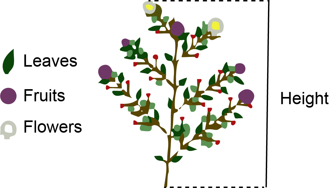
The green parts represent leaves, the purple circles represent fruits, and the white circles represent flowers. You can measure the following response (dependent) variables:
1. Height: You can use a ruler to measure height on your screen.
2. Growth rate: If you measure height over time, you can calculate absolute growth rate (AGR) as:
\[ \text{AGR}=\frac{H_{2}-H_{1}}{t_{2}-t_{1}} \] where \(H_{1}\) is the initial measured height at time \(t_{1}\), and \(H_{2}\) is the final or next measured height at time \(t_{2}\). Make sure your screen is the same size each time so that your measurements are consistent over time.
3. Number of leaves: Count the number of green parts at a specific time point.
4. Number of fruits: Count the number of purple circles at a specific time point.
5. Number of flowers: Count the number of white circles at a specific time point.
6. Branches: Count the number of diverging branches from the main stem at a specific time point.
7. Time to first flowering: The time difference from the start of the experiment to the first observed flower in the experimental plot.
8. Time to first fruit: The time difference from the start of the experiment to the first observed fruit in the experimental plot.
9. Yield: Once harvested, you will get a number in the “Harvest” tab (Table 2). The data table includes the date of harvest, the row and column of the plot, and the yield or biomass (g). Once harvested, the plant does not grow again (harvesting is a one-time, destructive measurement), so plan carefully when to harvest.
| Date | Row | Column | Yield |
|---|---|---|---|
| 01/064 | 1 | 1 | 320 |
| 02/064 | 1 | 2 | 269 |
| 03/064 | 1 | 3 | 327 |
| 04/064 | 1 | 4 | 390 |
| 05/064 | 1 | 5 | 307 |
I have no idea what the red circles are. You can count them and assign a name to them if you like (e.g. berries, fungal pathogen).
Which analysis suits which measurement?
Think about how you will analyse each response before you start your experiment.
| Response | Type of data | Workshop |
|---|---|---|
| Height, growth rate, yield (biomass) | Continuous | t-test / ANOVA (Week 5), regression (Week 7) |
| Number of leaves, flowers, fruits or branches | Counts | GLM for counts (Week 8) |
| Flowered or not, fruited or not | Binary (yes/no) | Logistic regression (Week 11) |
| Height measured repeatedly on the same plots | Repeated measures | Mixed-effects model (Week 12) |
| Time to first flowering or fruiting | Time-to-event (plots that never flowered are censored) | Survival analysis (Week 13) |