Week 9 (study week): Downloading and mapping species occurrence data
This is an optional tutorial for anyone working with species occurrence or other spatial data.
Note
This tutorial is optional and not assessed, and it will not be in the exam. Work through it in your own time if maps are relevant to your project. It was inspired by Amanda Buyan and Dax Kellie’s tutorials for the Atlas of Living Australia (ALA).
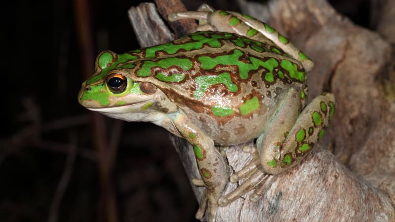
Maps are one of the most useful tools an ecologist has. A quick map of species observations shows where a species has been recorded, the extent of your data, and possible errors (e.g. a frog recorded in the ocean). In this tutorial you will download records of the motorbike frog (Litoria moorei) in Western Australia since 2000 from FrogID, and map them.
The motorbike frog (Litoria moorei). Photo: Stephen Mahony.
Code
# Week 9 workshop (optional) - Spatial data# Written by Nicholas Wu, 1234578, 22/04/2027# Install these packages once, in the console, if needed:# install.packages(c("galah", "sf", "ozmaps", "leaflet"))library(tidyverse) # data wrangling and plottinglibrary(galah) # download data from the Atlas of Living Australialibrary(sf) # work with spatial (map) datalibrary(patchwork) # combine plotslibrary(ozmaps) # outlines of Australian states
Download the data
Search for a taxon
galah::search_taxa() checks that the ALA recognises your species name and shows its full taxonomy. It is worth doing this even when you know the scientific name.
Code
galah::search_taxa("Litoria moorei")
# A tibble: 1 × 15
search_term scientific_name scientific_name_author…¹ taxon_concept_id rank
<chr> <chr> <chr> <chr> <chr>
1 Litoria moorei Litoria moorei (Copland, 1957) https://biodive… spec…
# ℹ abbreviated name: ¹scientific_name_authorship
# ℹ 10 more variables: match_type <chr>, vernacular_name <chr>, issues <chr>,
# kingdom <chr>, phylum <chr>, class <chr>, order <chr>, family <chr>,
# genus <chr>, species <chr>
Search for fields
Next, find the names of the fields (columns) you want to filter on: here year, state and data source. galah::search_all() searches the available fields:
Code
galah::search_all(fields, "year")
# A tibble: 8 × 3
  id                  description            type
  <chr>               <chr>                  <chr>
1 year                Year                   fields
2 raw_year            Year (unprocessed)     fields
3 endDayOfYear        End Day Of Year        fields
4 startDayOfYear      Start Day Of Year      fields
5 occurrenceYear      Date (by year)         fields
6 raw_endDayOfYear    <NA>                   fields
7 raw_startDayOfYear  <NA>                   fields
8 namePublishedInYear Name Published In Year fields
Code
galah::search_all(fields, "states")
# A tibble: 6 × 3
  id       description                            type
  <chr>    <chr>                                  <chr>
1 cl2013   ASGS Australian States and Territories fields
2 cl22     Australian States and Territories      fields
3 cl927    States including coastal waters        fields
4 cl10925  PSMA States (2016)                     fields
5 cl11174  States and Territories 2021            fields
6 cl110925 PSMA States - Abbreviated (2016)       fields
Code
galah::search_all(fields, "resource")
# A tibble: 5 × 3
  id                     description                                    type
  <chr>                  <chr>                                          <chr>
1 cl11160                Natural Resource Management (NRM) Regions 2023 fields
2 dataResourceUid        Dataset                                        fields
3 dataResourceName       Dataset                                        fields
4 relatedResourceID      Related Resource ID                            fields
5 relationshipOfResource Relationship Of Resource                       fields
galah::show_values() lists the possible values of a field. The field cl22 contains Australian states and territories:
Code
options(timeout =120) # allow more time for the downloadgalah::search_all(fields, "cl22") %>% galah::show_values()
# A tibble: 11 × 1
   cl22
   <chr>
 1 New South Wales
 2 Victoria
 3 Queensland
 4 Western Australia
 5 South Australia
 6 Northern Territory
 7 Tasmania
 8 Australian Capital Territory
 9 Macquarie Island
10 Coral Sea Islands
11 Ashmore and Cartier Islands
Download observations
Always count the records before downloading them, so you do not accidentally download millions of rows:
Code
galah::galah_call() %>%# start a query galah::galah_identify("Litoria moorei") %>%# motorbike frog galah::galah_filter(year >=2000, # since 2000 cl22 =="Western Australia", # in Western Australia dataResourceName =="FrogID") %>%# recorded by FrogID galah::atlas_counts() # count the records
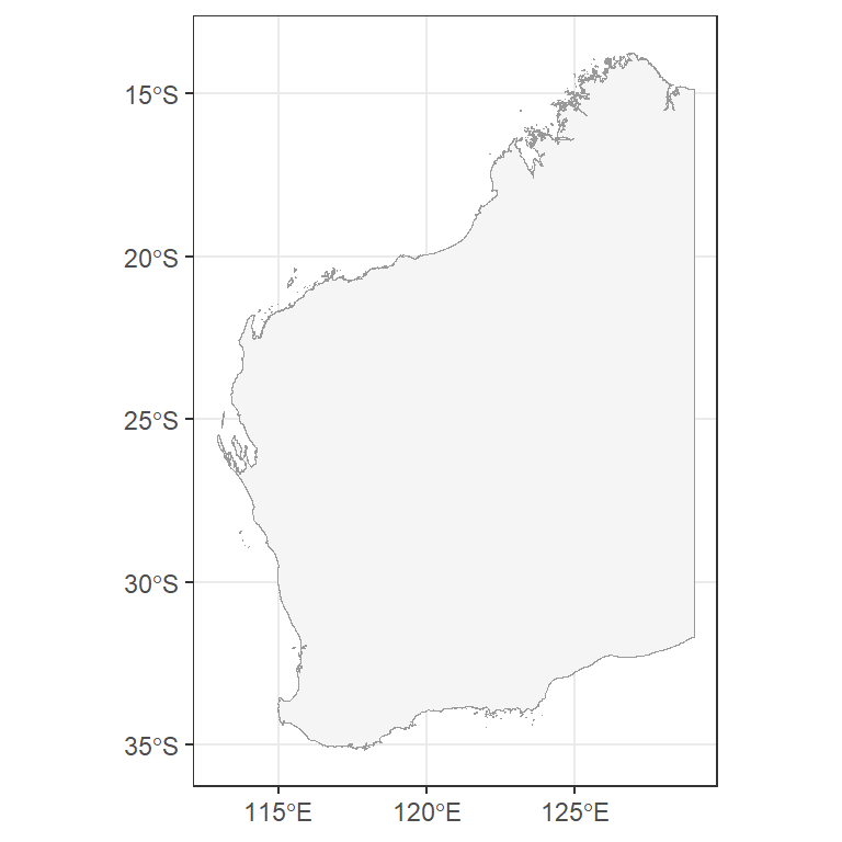
The ozmaps package contains outlines of Australian states. Keep Western Australia and plot it with ggplot2::geom_sf(), which draws spatial (sf) objects.
Code
au_map <- ozmaps::ozmap_data("abs_ste") # Australian stateswa_map <- au_map %>% dplyr::filter(NAME =="Western Australia") # keep WA onlyggplot2::ggplot() + ggplot2::geom_sf(data = wa_map, colour ="grey60", fill ="#F5F5F5") + ggplot2::theme_bw()
Coordinate reference systems
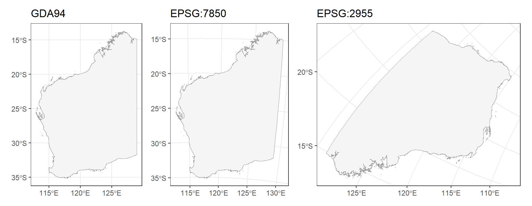
The Earth is round but maps are flat, so every map uses a coordinate reference system (CRS) to flatten it. Our WA outline uses GDA94:
Code
sf::st_crs(wa_map)$input
[1] "EPSG:4283"
The same outline looks different in different CRSs. sf::st_transform() changes the CRS:
Code
crs_gda94 <- ggplot2::ggplot(wa_map) + ggplot2::geom_sf(colour ="grey60", fill ="#F5F5F5") + ggplot2::labs(title ="GDA94") + ggplot2::theme_bw()crs_wa <- wa_map %>% sf::st_transform(crs =7850) %>%# a projection designed for WA (GDA2020 / MGA zone 50) ggplot2::ggplot() + ggplot2::geom_sf(colour ="grey60", fill ="#F5F5F5") + ggplot2::labs(title ="EPSG:7850") + ggplot2::theme_bw()crs_canada <- wa_map %>% sf::st_transform(crs =2955) %>%# a projection designed for Canada! ggplot2::ggplot() + ggplot2::geom_sf(colour ="grey60", fill ="#F5F5F5") + ggplot2::labs(title ="EPSG:2955") + ggplot2::theme_bw()crs_gda94 + crs_wa + crs_canada
Always check that all your spatial layers use the same CRS before combining them.
Add the observations
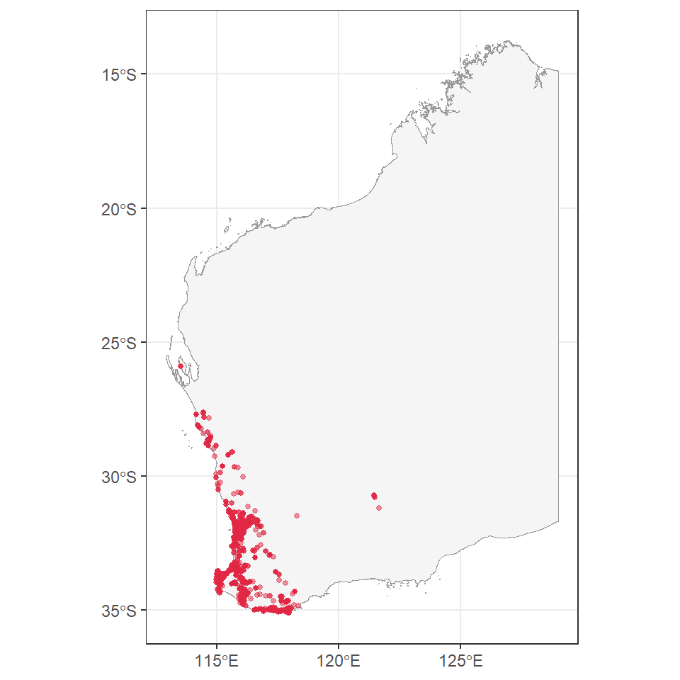
Plot the outline, then add the records as points (longitude on the x-axis, latitude on the y-axis):
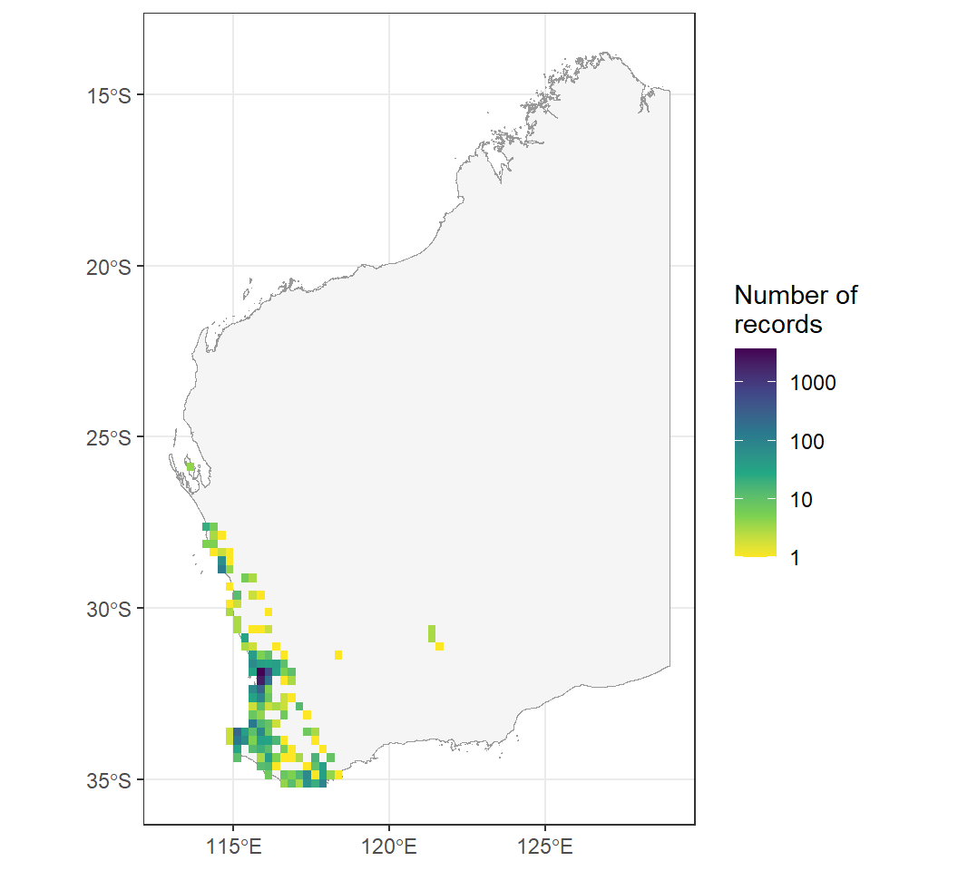
With thousands of overlapping points it is hard to see where records are concentrated. ggplot2::geom_bin_2d() counts the records in grid cells instead:
Code
ggplot2::ggplot() + ggplot2::geom_sf(data = wa_map, colour ="grey60", fill ="#F5F5F5") + ggplot2::geom_bin_2d(data = frogs, ggplot2::aes(x = decimalLongitude, y = decimalLatitude),binwidth =0.25) +# grid cells of 0.25 degrees ggplot2::scale_fill_viridis_c(trans ="log10", direction =-1) + ggplot2::labs(x =NULL, y =NULL, fill ="Number of\nrecords") + ggplot2::theme_bw()
Most records come from around Perth, where most people live and record frogs.
Interactive map
The leaflet package makes interactive maps you can zoom and pan. Hover over a point to see the date of the record.
Code
# Convert the table to a spatial object with longitude/latitude coordinates (CRS 4326)frogs_sf <- frogs %>% tidyr::drop_na(decimalLongitude, decimalLatitude) %>% sf::st_as_sf(coords =c("decimalLongitude", "decimalLatitude"), crs =4326)leaflet::leaflet() %>% leaflet::addTiles() %>%# background map leaflet::addCircles(data = frogs_sf,label =~as.character(eventDate),color ="#e12744")
Seasonality
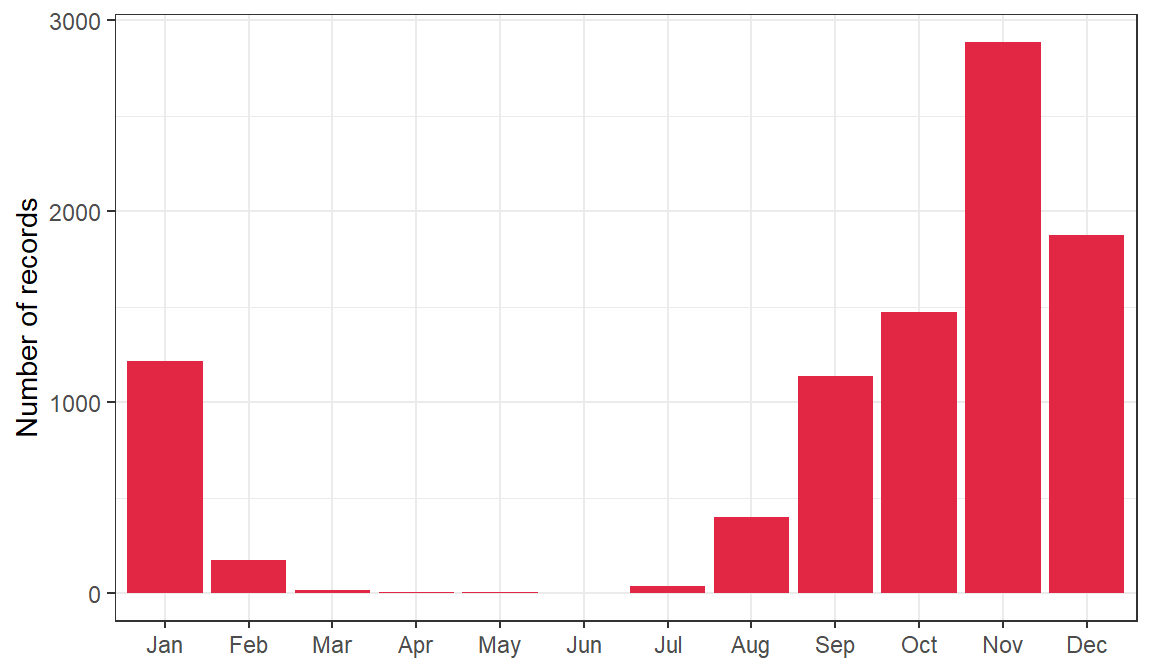
galah::galah_group_by() counts records per month without downloading them all:
ImportantCitizen science records are not standardised surveys
ALA records come from citizen scientists and researchers. Recording effort is not standardised: it depends on when and where people go out, which is especially true for rare species. A month with few records may mean fewer frogs calling, or fewer people listening. This kind of plot only shows real seasonal activity if survey effort is the same across the year. Remember from Research Design: “not recorded” is not the same as “absent”.
Types of spatial data
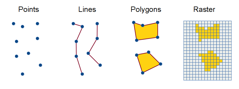
Spatial data come in two main forms:
Vector data are made of points (e.g. survey sites, occurrence records), lines (e.g. rivers, roads) and polygons (e.g. reserves, lakes, state boundaries). This tutorial used points and polygons.
Raster data are grids of cells, each with a value, used for continuous variables such as rainfall, temperature, elevation or vegetation cover.
Vector data are points, lines and polygons. Raster data are grids of cells.
Common mistakes
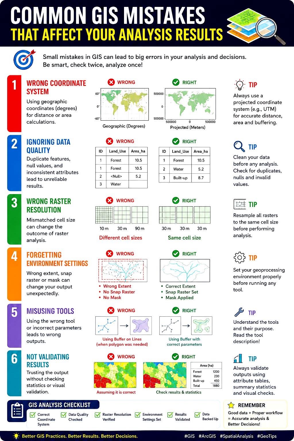
Check the quality of spatial data before plotting and analysing them. This tutorial does not cover spatial data cleaning, but here are common problems to look out for:
Common errors in species occurrence data.
Analysing spatial data
Spatial analysis is beyond this unit, but here are some possibilities:
Spatially explicit regression: sites close together tend to be similar (spatial autocorrelation), which breaks the independence assumption. Spatial models account for this. See Coding Club’s spatial modelling tutorial.
Species distribution models relate occurrence records to environmental predictors (climate, soil, habitat) to predict where a species could occur. They are used in conservation planning and to predict the effects of climate change and the spread of invasive species.