1  Quality Check

Week 1: Quality checks and data exploration

In this workshop you will learn how to check the quality of raw data after you import it into R, and how to fix common errors. Workshop materials are available in the GitHub repository ECS200.

All statistical techniques have in common the problem of ‘rubbish in, rubbish out’.

TipLearning outcomes

By the end of this workshop you should be able to:

  1. Check that each column of a dataset has been imported as the right type.
  2. Find and deal with missing values, duplicates and inconsistent labels.
  3. Use plots to find outliers and decide whether they are errors.
  4. Save a cleaned dataset for later analysis.

Background

How do we know the data are ready for analysis? Before any analysis, check the raw data for the following:

  • Data structure and types: is each column the type you expect (number, category, text, date)? Use str() or dplyr::glimpse().
  • Missing values: where are they, and how many? Use colSums(is.na()) or visdat::vis_miss().
  • Duplicates: are any rows accidentally entered twice?
  • Categorical variables: are categories spelt consistently (e.g. “Male”, “male” and “M” are three different categories to R)?
  • Outliers or impossible values: negative lengths, a 50 kg frog, a date in the future.
  • Column names: meaningful, with no spaces or special characters.
  • Extra rows or columns: notes, totals or empty columns copied from a spreadsheet.

These checks make sure your data are reliable and suitable for analysis, and they make you a trustworthy researcher.

The tidyverse

In this unit we use the tidyverse style of coding. The tidyverse is a collection of R packages for importing, cleaning, transforming and plotting data that share the same grammar, so once you learn one package the others feel familiar. It is widely used in ecology because ecological data are often large and messy, collected across space and time, and have replicates nested within sites.

Before we start

Create a new R script (File > New File > R Script). At the top, write the name of the workshop, your name, student number and the date. Do this every time you start a new script.

Code
# Week 1 workshop - Data quality check
# Written by Nicholas Wu, 1234578, 25/02/2027

Download the data and save it in the data folder inside your workshop folder.

plant_calcium.csv

Exercise (5 min)

🧪 Set up your workflow

Load the tidyverse package and the visdat package (for visualising missing data), set your working directory, and import plant_calcium.csv with readr::read_csv(). Call the imported object plant_calcium_data.

Details on installing and loading packages, setting your working directory and importing a CSV file are in the Introduction to R.

Show answer
Code
# Install packages (only once, in the console)
# install.packages("visdat")

# Load packages
library(tidyverse)
library(visdat)

# Set your working directory to your workshop folder
# setwd("C:/Users/YOUR-NAME/Documents/ECS200")

# Import the CSV file from the data folder
plant_calcium_data <- readr::read_csv("data/plant_calcium.csv")

The dataset contains sugar maple seedlings from a calcium-treated watershed (W1) and an untreated Reference watershed at Hubbard Brook, USA. You will learn more about the study in Week 2.

Step 1: Data quality check

1.1. Initial check

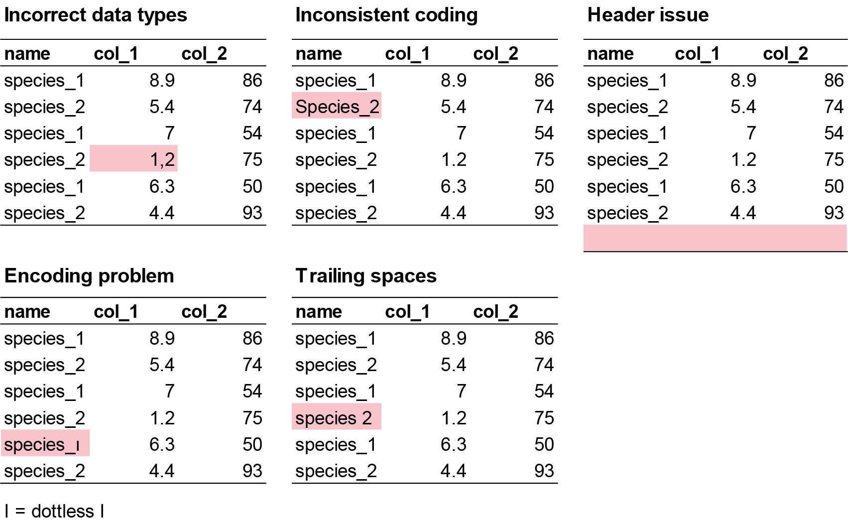
First, check that every variable was imported as the right type. Common problems include:

  • Incorrect data types: a numeric column is read as text (chr) because it contains a symbol, a word, a comma instead of a decimal point, or an empty string.
  • Inconsistent coding: one category spelt several ways (“Male”, “male”, “M”), which R treats as different categories.
  • Header issues: a missing header row, or extra rows of notes at the top or bottom of the file.
  • Encoding problems: special characters (e.g. °, µ, accents) that display incorrectly.
  • Trailing spaces: “site A” and “site A” are different to R.

Code
# Check the structure of your data (two ways to do the same thing)
str(plant_calcium_data)
spc_tbl_ [359 × 11] (S3: spec_tbl_df/tbl_df/tbl/data.frame)
 $ year               : num [1:359] 2003 2003 2003 2003 2003 ...
 $ watershed          : chr [1:359] "Reference" "Reference" "Reference" "Reference" ...
 $ elevation          : chr [1:359] "Low" "Low" "Low" "Low" ...
 $ transect           : chr [1:359] "R1" "R1" "R1" "R1" ...
 $ sample             : num [1:359] 1 2 3 4 5 6 7 8 9 10 ...
 $ stem_length        : num [1:359] 86.9 114 83.5 68.1 72.1 77.7 85.5 81.6 92.9 59.6 ...
 $ leaf1area          : num [1:359] 13.84 14.57 12.45 9.97 6.84 ...
 $ leaf2area          : num [1:359] 12.13 15.27 9.73 10.07 5.48 ...
 $ leaf_dry_mass      : num [1:359] 0.0453 0.0476 0.0423 0.0397 0.0204 0.0317 0.0382 0.0179 0.0286 0.0125 ...
 $ stem_dry_mass      : num [1:359] 0.03 0.0338 0.0248 0.0194 0.018 0.0246 0.0316 0.015 0.0291 0.0149 ...
 $ corrected_leaf_area: num [1:359] 29.1 33 25.3 23.2 15.5 ...
 - attr(*, "spec")=
  .. cols(
  ..   year = col_double(),
  ..   watershed = col_character(),
  ..   elevation = col_character(),
  ..   transect = col_character(),
  ..   sample = col_double(),
  ..   stem_length = col_double(),
  ..   leaf1area = col_double(),
  ..   leaf2area = col_double(),
  ..   leaf_dry_mass = col_double(),
  ..   stem_dry_mass = col_double(),
  ..   corrected_leaf_area = col_double()
  .. )
 - attr(*, "problems")=<pointer: 0x0000020b3f1fd890> 
Code
dplyr::glimpse(plant_calcium_data)
Rows: 359
Columns: 11
$ year                <dbl> 2003, 2003, 2003, 2003, 2003, 2003, 2003, 2003, 20…
$ watershed           <chr> "Reference", "Reference", "Reference", "Reference"…
$ elevation           <chr> "Low", "Low", "Low", "Low", "Low", "Low", "Low", "…
$ transect            <chr> "R1", "R1", "R1", "R1", "R1", "R1", "R1", "R1", "R…
$ sample              <dbl> 1, 2, 3, 4, 5, 6, 7, 8, 9, 10, 11, 12, 13, 14, 15,…
$ stem_length         <dbl> 86.9, 114.0, 83.5, 68.1, 72.1, 77.7, 85.5, 81.6, 9…
$ leaf1area           <dbl> 13.837, 14.572, 12.451, 9.974, 6.838, NA, NA, 5.83…
$ leaf2area           <dbl> 12.130, 15.267, 9.731, 10.068, 5.480, 7.643, 9.233…
$ leaf_dry_mass       <dbl> 0.0453, 0.0476, 0.0423, 0.0397, 0.0204, 0.0317, 0.…
$ stem_dry_mass       <dbl> 0.0300, 0.0338, 0.0248, 0.0194, 0.0180, 0.0246, 0.…
$ corrected_leaf_area <dbl> 29.104, 32.976, 25.319, 23.179, 15.455, 20.440, 21…
Code
# Summary of every variable (min, max, mean, number of NAs...)
summary(plant_calcium_data)
      year          watershed       elevation        transect       sample     
 Min.   :2003   Length   :359   Length   :359   Length   :359   Min.   : 1.00  
 1st Qu.:2003   N.unique :  2   N.unique :  2   N.unique : 12   1st Qu.: 5.50  
 Median :2003   N.blank  :  0   N.blank  :  0   N.blank  :  0   Median :10.00  
 Mean   :2003   Min.nchar:  2   Min.nchar:  3   Min.nchar:  2   Mean   :10.47  
 3rd Qu.:2004   Max.nchar:  9   Max.nchar:  3   Max.nchar:  4   3rd Qu.:15.00  
 Max.   :2004                   NAs      :119                   Max.   :20.00  
                                                                               
  stem_length       leaf1area        leaf2area       leaf_dry_mass    
 Min.   : 52.70   Min.   : 2.480   Min.   :  0.000   Min.   :0.01170  
 1st Qu.: 75.65   1st Qu.: 8.792   1st Qu.:  8.802   1st Qu.:0.03975  
 Median : 85.70   Median :11.616   Median : 11.275   Median :0.05590  
 Mean   : 86.86   Mean   :11.713   Mean   : 12.024   Mean   :0.06368  
 3rd Qu.: 97.05   3rd Qu.:13.837   3rd Qu.: 14.340   3rd Qu.:0.07855  
 Max.   :132.30   Max.   :26.952   Max.   :100.372   Max.   :0.38700  
                  NAs    :126      NAs    :117                        
 stem_dry_mass     corrected_leaf_area
 Min.   :0.00790   Min.   : 9.597     
 1st Qu.:0.02360   1st Qu.:21.180     
 Median :0.03320   Median :25.950     
 Mean   :0.04506   Mean   :26.687     
 3rd Qu.:0.05820   3rd Qu.:31.751     
 Max.   :0.15000   Max.   :55.874     
                   NAs    :119        

For small datasets like the ones in this workshop, it is often easiest to fix mistakes in Excel and import the CSV again. Fixing them in R is better practice, though, because the code records exactly what you changed. For example, suppose you have three sites (A, B and C) but one was mislabelled “E”. dplyr::if_else() replaces values that match a condition:

Code
# Example data with sites A, B and C, but one site was mislabelled as E
fake_data <- data.frame(
  site      = c("A", "A", "A", "B", "E", "B", "C", "C", "C"),
  species_1 = c(3, 7, 5, 2, 9, 4, 6, 1, 8)
)

fake_data %>%
  dplyr::mutate(site = dplyr::if_else(site == "E", "B", site)) # if site is "E" make it "B", otherwise keep it
  site species_1
1    A         3
2    A         7
3    A         5
4    B         2
5    B         9
6    B         4
7    C         6
8    C         1
9    C         8

If a number was typed as a word (e.g. “nine” instead of 9), the whole column is read as text. Fix the value, then convert the column to numeric with as.numeric():

Code
# Example data where one count was typed as a word
fake_data <- data.frame(
  site      = c("A", "A", "A", "B", "B", "B", "C", "C", "C"),
  species_1 = c(3, 7, 5, 2, "nine", 4, 6, 1, 8)
)

# Replace "nine" with "9", then change species_1 from text to numbers
fake_clean_data <- fake_data %>%
  dplyr::mutate(species_1 = dplyr::if_else(species_1 == "nine", "9", species_1),
                species_1 = as.numeric(species_1))

# Check that species_1 is now numeric (<dbl>)
dplyr::glimpse(fake_clean_data)
Rows: 9
Columns: 2
$ site      <chr> "A", "A", "A", "B", "B", "B", "C", "C", "C"
$ species_1 <dbl> 3, 7, 5, 2, 9, 4, 6, 1, 8

Exercise (5 min)

🧪 Find the three problems in this dataset

Code
fake_data <- data.frame(
  site = c("A", "B", "C", "A", "B", "A", "B", "C", "a", "B", "A", "B", "A", "B", "C", "C",
           "B", "A", "A", "C", "B", "C", "C", "A", "A", "A", "A", "B", "C", "C", "C"),
  species_1 = c(7, 25, 30, 50, 38, 13, 5, 31, 34, 22, 41, 25, 22, 37, 39, 13,
                45, 10, 40, 7, 28, 36, 19, 2, 12, 5, 16, 38, 27, 44, 44),
  species_2 = c(9.3, 8.6, 0.8, 7.5, 9, 9.1, 4.3, 8.6, 0.1, 7.8, 1.2, 6.2, 0.4, 0.4, 7.4, 1.9,
                8.3, 7.8, 2.9, 9.3, 9.1, 2.3, 6.3, 8.5, 6.5, 6.6, "1,7", 1.8, 8.4, 4.7, 4.7),
  species_3 = c(190, 160, 70, 430, 310, 99, 530, 420, 371, 357, 198, 171, 463, 124, 254, 484,
                435, 409, 122, 305, 410, 162, 473, 200, 401, 273, 421, 419, 293, 487, 487),
  species_4 = c(2, 0, 4, 8, 6.7, 3, 7.2, 4.3, 2, NA, 10, 10, 6, 4, 8, 1.7,
                1, 0, NA, 4, 6, 8.2, 10, 6, 2, 5, 10, 7, NA, NA, NA)
)
Show answer
  1. site has an inconsistent label: “a” should be “A”. (site should also be converted to a factor before analysis.)
  2. species_2 was read as text (chr) because one value was typed as “1,7” instead of 1.7.
  3. species_4 has 5 missing values (NA).

1.2. Identify missing values

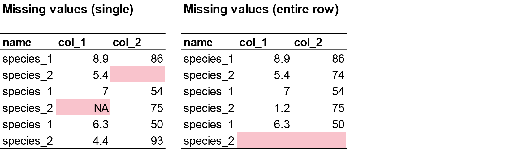
Missing data can appear as blank cells, “NA”, “.”, “-” or other placeholders. If they are not handled properly, they cause errors or misleading results.

Code
# Count the missing values in each column
colSums(is.na(plant_calcium_data))
               year           watershed           elevation            transect 
                  0                   0                 119                   0 
             sample         stem_length           leaf1area           leaf2area 
                  0                   0                 126                 117 
      leaf_dry_mass       stem_dry_mass corrected_leaf_area 
                  0                   0                 119 

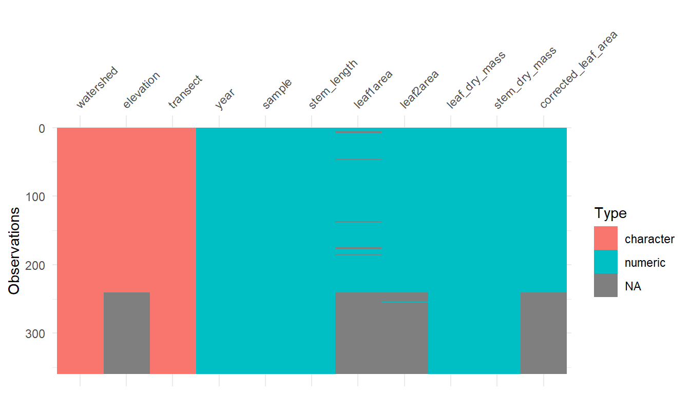
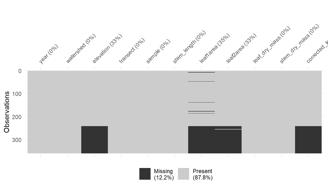
visdat::vis_dat() shows the whole data frame at once, coloured by the type of each column, with missing values in grey. visdat::vis_miss() shows only whether values are missing, and the percentage missing in each column.

Code
visdat::vis_dat(plant_calcium_data)

Code
visdat::vis_miss(plant_calcium_data)

What should you do with missing values? It depends on which columns they are in and on your question. tidyr::drop_na() removes rows with missing values:

Code
# Removes every row that has an NA in ANY column. Usually too harsh: here it
# would remove all of 2004, because elevation was not recorded that year.
plant_data_all_complete <- plant_calcium_data %>%
  tidyr::drop_na()

# Removes rows with an NA in the leaf2area column only. Use this when you are
# about to analyse leaf2area.
plant_data_clean <- plant_calcium_data %>%
  tidyr::drop_na(leaf2area)

# Compare the number of rows
nrow(plant_calcium_data)
[1] 359
Code
nrow(plant_data_all_complete)
[1] 233
Code
nrow(plant_data_clean)
[1] 242

Only remove missing values from the columns you actually need. Remember that a missing value (NA) is not the same as a zero. See Research Design.

Exercise (5 min)

🧪 Identify and handle missing values in fake_data

  • Which column contains missing values, and how many are there?
  • Remove the rows with missing values in that column, and call the result fake_data_clean.
  • Check the result with visdat::vis_miss(fake_data_clean).
Show answer
Code
# Count missing values in each column: species_4 has 5
colSums(is.na(fake_data))

# Remove rows where species_4 is missing
fake_data_clean <- fake_data %>%
  tidyr::drop_na(species_4)

# Check that the NAs have gone
visdat::vis_miss(fake_data_clean)

1.3. Checking duplicates

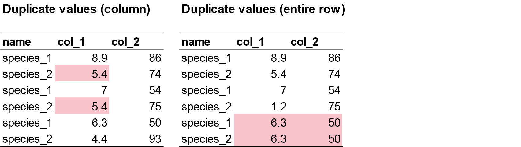
There are two kinds of duplicates:

  1. Row duplicates: two rows are identical in every column. This is almost always an error (e.g. copy and paste) and should be removed.
Code
# Number of rows that are exact copies of an earlier row
sum(duplicated(plant_calcium_data))
[1] 0
Code
# Show the duplicated rows (none here, so this returns an empty table)
plant_calcium_data[duplicated(plant_calcium_data), ]
# A tibble: 0 × 11
# ℹ 11 variables: year <dbl>, watershed <chr>, elevation <chr>, transect <chr>,
#   sample <dbl>, stem_length <dbl>, leaf1area <dbl>, leaf2area <dbl>,
#   leaf_dry_mass <dbl>, stem_dry_mass <dbl>, corrected_leaf_area <dbl>

There are no duplicated rows in plant_calcium_data.

  1. Value duplicates: the same value appears more than once in a column. This is usually real (e.g. two seedlings with a leaf mass of 0.03 g, especially after rounding). Be suspicious if there is a pattern, e.g. 2, 2, 6, 1, 2, 2, 9, 4, 2, 2, which suggests values were copied into the next row by accident. You, the researcher, have to decide whether duplicated values are real.
Code
# Number of values in leaf_dry_mass that repeat an earlier value
sum(duplicated(plant_calcium_data$leaf_dry_mass))
[1] 51

There are 51 repeated values in leaf_dry_mass, which is expected for masses rounded to four decimal places.

Exercise (3 min)

🧪 Find the duplicate row in fake_data

  • Which row is duplicated?
  • Remove it, either in Excel (easy) or with dplyr::distinct() (challenge).
  • Are there duplicated values in the species columns? Are they likely to be real?
Show answer
Code
sum(duplicated(fake_data))      # 1 duplicated row
fake_data[duplicated(fake_data), ] # row 31 is a copy of row 30

# Keep only unique rows
fake_data_unique <- fake_data %>%
  dplyr::distinct()

# Repeated values within each column (common for counts, so probably real)
sum(duplicated(fake_data$species_1))
sum(duplicated(fake_data$species_3))

Step 2: Visualising data

2.1. Check for outliers

Outliers are not automatically “bad”, but they can cause problems. They can:

  1. Distort results: a single extreme value can drag the mean, inflate the variation, and change the slope of a regression line.
  2. Hide patterns: one extreme value squashes the rest of the data on a plot.
  3. Reveal errors: data entry mistakes (typing 1000 instead of 100), faulty equipment, or mixed-up units (metres and centimetres).

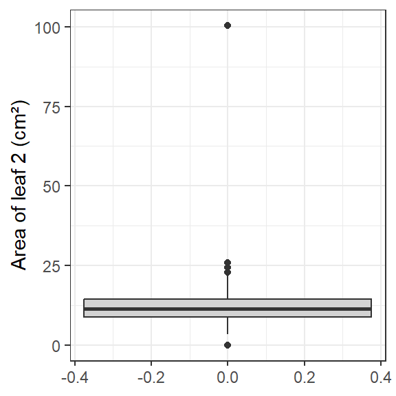
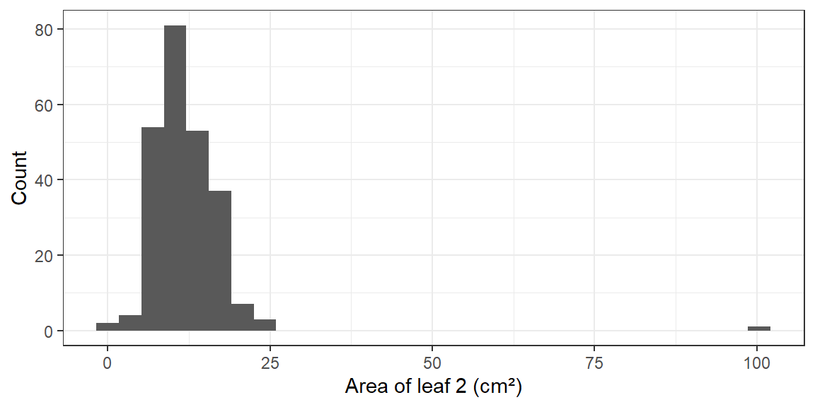
Two simple plots will reveal most outliers.

There is one clear outlier above 100 cm2. Every other leaf is smaller than 25 cm2. You can list potential outliers with the interquartile range (IQR) rule:

Code
# Quartiles and interquartile range of leaf2area
q1  <- quantile(plant_data_clean$leaf2area, 0.25)
q3  <- quantile(plant_data_clean$leaf2area, 0.75)
iqr <- q3 - q1

# Rows with leaf2area more than 1.5 x IQR below Q1 or above Q3
plant_data_clean %>%
  dplyr::filter(leaf2area < q1 - 1.5 * iqr | leaf2area > q3 + 1.5 * iqr)
# A tibble: 6 × 11
   year watershed elevation transect sample stem_length leaf1area leaf2area
  <dbl> <chr>     <chr>     <chr>     <dbl>       <dbl>     <dbl>     <dbl>
1  2003 W1        Low       W1-6         16       110.       NA        24.2
2  2003 W1        Low       W1-6         19       101.       21.8      22.9
3  2003 W1        Mid       W1-3         17        87.9      27.0      25.8
4  2003 W1        Mid       W1-5         20        67.9      10.1     100. 
5  2004 Reference <NA>      R1           14        57        NA         0  
6  2004 Reference <NA>      R1           15        99        NA         0  
# ℹ 3 more variables: leaf_dry_mass <dbl>, stem_dry_mass <dbl>,
#   corrected_leaf_area <dbl>

The IQR rule flags a few leaves, but only the 100 cm2 leaf is biologically unrealistic for a sugar maple seedling, so it is almost certainly a data entry error. Always use your biological knowledge (and the literature) to decide. Do not remove values just because a rule flags them.

2.2. Are the data normally distributed?

Many statistical tests (t-tests, ANOVA, linear regression) assume that the data (or, more precisely, the model’s residuals) are roughly normally distributed, with constant variance. If the data are strongly skewed, have outliers or have unequal variances, those tests can give biased estimates and wrong conclusions. You will learn how to check this properly in Weeks 5 and 7, and how to transform data in Week 2.

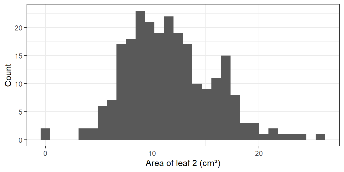
Let’s look at leaf2area again after removing the impossible value.

Code
# Remove the data-entry error (the one leaf above 100 cm2)
plant_data_clean <- plant_data_clean %>%
  dplyr::filter(leaf2area < 100)

ggplot2::ggplot(plant_data_clean, ggplot2::aes(x = leaf2area)) +
  ggplot2::geom_histogram(bins = 30) +
  ggplot2::labs(x = "Area of leaf 2 (cm²)", y = "Count") +
  ggplot2::theme_bw()

The distribution is now roughly symmetrical and bell-shaped.

Assessment

Task to complete before the end of the workshop.

week01_assessment.R plant_calcium_task.csv

plant_calcium_task.csv is a modified version of plant_calcium.csv. Some errors have been introduced. Run a quality check, fix the problems, and save a clean version that you will use again in Weeks 2 and 3.

To make it easier, here are hints about where the errors are. With your own data, you will need to check everything thoroughly.

  1. One of the numeric columns has missing values. Decide whether you really need to remove these rows, and explain why.
  2. One of the categorical variables has an inconsistent label. Correct it. You can do this in Excel or in R, but say in a comment which one you used.
  3. Two numeric columns each contain an extreme value. One is biologically realistic and the other is a data entry mistake. Decide which is the mistake and remove it.
  4. Convert watershed and transect to factors.
  5. Plot the distribution of stem_dry_mass in your clean data as a density plot (ggplot2::geom_density()).
  6. Interpretation: in two or three sentences (as comments), explain how you decided which extreme value was an error, and why it matters to remove it before analysing the data.
  7. Save the clean data as plant_task_data_clean.csv in your data folder:
Code
# Save the cleaned data (it will be saved inside the data folder)
readr::write_csv(plant_task_data_clean, "data/plant_task_data_clean.csv")

Submit one R script (.R) before the end of the class. Write your answers to written questions as # comments next to the code that produced them.

Score What it looks like
0 No submission or no attempt.
0.25 Submitted, but a very poor attempt (e.g. incomplete, or lots of gaps).
0.5 Most questions answered, or all answered but most annotations missing.
0.75 All questions answered, but some annotations missing or some answers incorrect.
1 Everything completed, with annotations on all code so the marker can follow it.

Tip: an annotation is a short # comment that says what the line does and why. For example: # remove the one plant with a stem dry mass of 7.4 g (data entry error).

For the adventurous

  • Write a single pipe that imports plant_calcium_task.csv, fixes the label, converts the categorical columns to factors and removes the error, all in one step.
  • Plot the density of stem_dry_mass separately for the two watersheds (hint: fill = watershed).

Additional resources